Exploring Graphs of Quadratic Functions 2

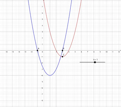
This GeoGebra example dynamically illustrates how changing the coefficients a, b, and c in the quadratic function y = ax² + bx + c affects the parabola's opening direction, axis of symmetry, and vertex position. Core mathematical concepts include the standard form of quadratic functions, completing the square, the discriminant, and transformations such as shifting and scaling. The construction uses the Point command to create key points A, B, and C, along with parameters a, b, c, p, q, k, and d (likely as sliders or numeric values) to update the graph in real time. It also highlights intersections with axes and the vertex locus. Suitable for middle-to-high school students learning quadratic function properties, as well as for classroom demonstrations or self-guided exploration of parameter effects.