
Exploring First, Second, and Mixed Partial Derivatives
Loading the math board and drawing, please wait…
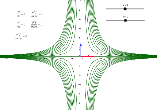
This example dynamically illustrates the concepts of first, second, and mixed partial derivatives. It involves the calculation of partial derivatives of multivariable functions and demonstrates their geometric meanings through vector and function objects. Commands like Vector, Derivative, and Sequence are used, suitable for university-level calculus courses.
GeoGebra Commands & Parameters
Vector((a, b), (a + 1.5, b)) → uVector((a, b), (a, b + 1.5)) → vDerivative(f(x, y), x) → fxDerivative(fx(x, y), y) → fxySequence(ImplicitCurve[f(x, y) - i], i, -10, 10) → list1Derivative(f(x, y), y) → fyDerivative(fx(x, y), x) → fxxDerivative(fy(x, y), y) → fyy
AI Drawing Prompt Reference
Draw the graph of a multivariable function and illustrate the geometric meaning of its first and second partial derivatives. Add two perpendicular vectors to the function graph, representing the rates of change in the x and y directions. Use curves to show the level sets of the function and different vectors to represent the first and second partial derivatives, demonstrating their relationship with the function graph.
The prompt above was compiled from the original drawing commands and is for reference only.