Contour Plots and Partial Derivatives Visualization

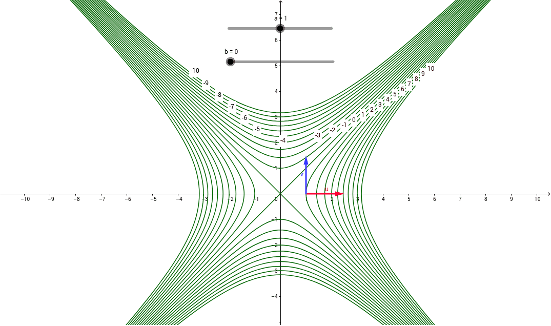
This example visually demonstrates the concept of partial derivatives through contour plots, illustrating how a multivariable function changes with respect to each variable. Key mathematical concepts include partial derivatives, contour lines, and the geometric interpretation of directional change. Constructed using GeoGebra commands Sequence and Vector, along with objects list1, list2, list3, the model builds layered data and vector representations to show function behavior. It is suitable for high school or early university calculus students seeking an intuitive understanding of partial derivatives and their applications.