
Exploring a Conformal Mapping: f(z)=2π / sqrt(9.82) z⁰·⁵
Loading the math board and drawing, please wait…
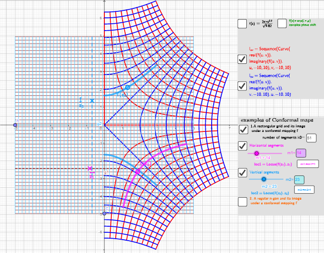
This example demonstrates the conformal mapping properties and graphical representation of the complex function f(z)=2π / sqrt(9.82) z⁰·⁵. Key mathematical concepts include complex functions, conformal mappings, similarity transformations, and polar coordinate transformations. The construction utilizes GeoGebra commands such as Point, Sequence, Locus, Textfield, Polygon, and Surface to visualize the function, its trajectory, and geometric shapes. Suitable for high school and advanced learners to understand the geometric meaning and transformation characteristics of complex functions.
GeoGebra Commands & Parameters
Point(yAxis) → CPoint(xAxis) → ASequence(Segment[A + (0, y(C) + (k * dy)), ((-x(A)), y(C) + (k * dy))], k, 0, k0) → l1, {10, 10, 10, 10, 10, 10, 10, 10, 10, 10, 10, 10, 10, 10, 10, 10, 10, 10, 10, 10, 10, 10, 10, 10, 10, 10, 10, 10, 10, 10, 10, 10, 10, 10, 10, 10, 10, 10, 10, 10, 10, 10, 10, 10, 10, 10, 10, 10, 10, 10, 10, 10}Point(g1) → z_1Point(l1) → ELocus(fz_{1}, z_1) → loc1Sequence(CurveCartesian[real(f(u, v)), imaginary(f(u, v)), u, -10, 10], v, -10, 10) → l_{uv}, {(real(f(u, -10)), imaginary(f(u, -10))), (real(f(u, -9)), imaginary(f(u, -9))), (real(f(u, -8)), imaginary(f(u, -8))), (real(f(u, -7)), imaginary(f(u, -7))), (real(f(u, -6)), imaginary(f(u, -6))), (real(f(u, -5)), imaginary(f(u, -5))), (real(f(u, -4)), imaginary(f(u, -4))), (real(f(u, -3)), imaginary(f(u, -3))), (real(f(u, -2)), imaginary(f(u, -2))), (real(f(u, -1)), imaginary(f(u, -1))), (real(f(u, 0)), imaginary(f(u, 0))), (real(f(u, 1)), imaginary(f(u, 1))), (real(f(u, 2)), imaginary(f(u, 2))), (real(f(u, 3)), imaginary(f(u, 3))), (real(f(u, 4)), imaginary(f(u, 4))), (real(f(u, 5)), imaginary(f(u, 5))), (real(f(u, 6)), imaginary(f(u, 6))), (real(f(u, 7)), imaginary(f(u, 7))), (real(f(u, 8)), imaginary(f(u, 8))), (real(f(u, 9)), imaginary(f(u, 9))), (real(f(u, 10)), imaginary(f(u, 10)))}Sequence(CurveCartesian[real(f(u, v)), imaginary(f(u, v)), v, -10, 10], u, -10, 10) → l_{vu}, {(real(f(-10, v)), imaginary(f(-10, v))), (real(f(-9, v)), imaginary(f(-9, v))), (real(f(-8, v)), imaginary(f(-8, v))), (real(f(-7, v)), imaginary(f(-7, v))), (real(f(-6, v)), imaginary(f(-6, v))), (real(f(-5, v)), imaginary(f(-5, v))), (real(f(-4, v)), imaginary(f(-4, v))), (real(f(-3, v)), imaginary(f(-3, v))), (real(f(-2, v)), imaginary(f(-2, v))), (real(f(-1, v)), imaginary(f(-1, v))), (real(f(0, v)), imaginary(f(0, v))), (real(f(1, v)), imaginary(f(1, v))), (real(f(2, v)), imaginary(f(2, v))), (real(f(3, v)), imaginary(f(3, v))), (real(f(4, v)), imaginary(f(4, v))), (real(f(5, v)), imaginary(f(5, v))), (real(f(6, v)), imaginary(f(6, v))), (real(f(7, v)), imaginary(f(7, v))), (real(f(8, v)), imaginary(f(8, v))), (real(f(9, v)), imaginary(f(9, v))), (real(f(10, v)), imaginary(f(10, v)))}Sequence(Segment[C + (x(A) + (k * dx), 0), (0, (-y(C))) + (x(A) + (k * dx), 0)], k, 0, k0) → l2, {9.92203865203867, 9.92203865203867, 9.92203865203867, 9.92203865203867, 9.92203865203867, 9.92203865203867, 9.92203865203867, 9.92203865203867, 9.92203865203867, 9.92203865203867, 9.92203865203867, 9.92203865203867, 9.92203865203867, 9.92203865203867, 9.92203865203867, 9.92203865203867, 9.92203865203867, 9.92203865203867, 9.92203865203867, 9.92203865203867, 9.92203865203867, 9.92203865203867, 9.92203865203867, 9.92203865203867, 9.92203865203867, 9.92203865203867, 9.92203865203867, 9.92203865203867, 9.92203865203867, 9.92203865203867, 9.92203865203867, 9.92203865203867, 9.92203865203867, 9.92203865203867, 9.92203865203867, 9.92203865203867, 9.92203865203867, 9.92203865203867, 9.92203865203867, 9.92203865203867, 9.92203865203867, 9.92203865203867, 9.92203865203867, 9.92203865203867, 9.92203865203867, 9.92203865203867, 9.92203865203867, 9.92203865203867, 9.92203865203867, 9.92203865203867, 9.92203865203867, 9.92203865203867}Point(g2) → z_{2}Locus(fz_{2}, z_{2}) → loc2Textfield(k0) → InputBox1Textfield(m1) → InputBox2Textfield(m2) → InputBox3Polygon(D, F, n) → poli1, s, l, J, N, R, V, H, I, K, L, t, f_1, j_1, n_1, s_1, i, j, kPoint(poli1) → z_3Locus(fz_{3}, z_3) → loc3Surface(f(u + (v * ί)), u, -2, 2, v, -2, 2) → pTextfield(φ) → InputBox4
AI Drawing Prompt Reference
Create a visualization of a conformal mapping for the complex function f(z)=2π/√9.82·z^0.5 in the complex plane. Include a set of curves obtained by mapping a domain grid: draw trajectory images for two families where the real part varies with fixed imaginary part, and where the imaginary part varies with fixed real part. Place reference points on the coordinate axes, add additional points used to trace mapped paths, and show the corresponding mapped loci/trajectories together. Include a few text labels and adjustable input fields for parameters controlling the sampling and curve construction, and add a simple surface/patch style element to emphasize the geometric representation of the mapping.
The prompt above was compiled from the original drawing commands and is for reference only.