
Explore Pythagorean Theorem: Dynamic Geometry Interactive
Loading the math board and drawing, please wait…
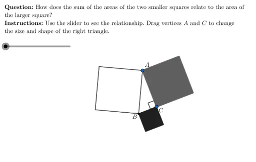
① This example dynamically demonstrates the geometric meaning of the Pythagorean theorem by showing the area relationship among squares built on the three sides of a right triangle. ② Core mathematical concepts include the Pythagorean theorem, equilateral triangles, arithmetic mean, orthocenter, and stochastic processes (for generating random triangles). ③ Construction highlights: using GeoGebra commands such as Circle, PointIn, CircleArc, Point, Vector, OrthogonalVector, Polygon, Intersect, and Angle to construct the right triangle and squares on its sides; a random process (TryAnother button) generates different triangles, with midpoints (MidBC etc.) and vector operations (e.g., vBCAB1) aiding the construction. ④ Suitable for middle and high school students learning the Pythagorean theorem, and useful for classroom demonstrations or self-exploration to deepen understanding through dynamic variation.
GeoGebra Commands & Parameters
Circle(B + (0, 6), 5) → bCircPointIn(bCirc) → ACircleArc(Midpoint[B, A], Rotate[B, 5°, Midpoint[B, A]], Rotate[A, (-(5°)), Midpoint[B, A]]) → cArcPoint(cArc) → CVector(B, C) → vACVector(A, C) → vBCOrthogonalVector(vBC) → pBCVector(B, A) → vABOrthogonalVector(vAB) → pABPolygon({A, A + vBC, A + vBC + pBC, A + pBC}) → quadBCLaTeX((((("\text{\textbf{Question: }" * MainInstruc) * "\\\textbf{Instructions: }") * SpecInstruc) * "}")) → allInstrucPolygon({B, B + vAC, B + vAC + pAC, B + pAC}) → quadACPolygon({B, B + vAB, B + vAB + pAB, B + pAB}) → quadABVector(MidBC, AB_v2) → vBCAB2Vector(MidBC, AB_v1) → vBCAB1Vector(MidBC, B) → vBCAVector(MidBC, A) → vBCBVector(MidAC, A) → vACBVector(MidAC, B) → vACAVector(MidAC, AB_v1) → vACAB1Vector(MidAC, AB_v2) → vACAB2Intersect(Ray[MidAC, Vector[(-vAB)]], Segment[B, AC_v2]) → AC_cIntersect(Ray[MidAC, vAB], Segment[C, AC_v1]) → AC_aIntersect(Ray[MidAC, pAB], quadAC) → AC_dPolygon({MidAC, AC_d, B, AC_c}) → qACcIntersect(Ray[MidAC, Vector[(-pAB)]], Segment[AC_v1, AC_v2]) → AC_bPolygon({MidAC, AC_c, AC_v2, AC_b}) → qACbPolygon({MidAC, AC_b, AC_v1, AC_a}) → qACaPolygon({MidAC, AC_a, C, AC_d}) → qACdIntersect(Ray[MidBC, vAB], Segment[A, BC_v1]) → BC_aIntersect(Ray[MidBC, Vector[(-pAB)]], Segment[BC_v1, BC_v2]) → BC_bIntersect(Ray[MidBC, Vector[(-vAB)]], Segment[C, BC_v2]) → BC_cIntersect(Ray[MidBC, pAB], Segment[A, C]) → BC_dPolygon({MidBC, BC_a, BC_v1, BC_b}) → qBCaPolygon({MidBC, BC_b, BC_v2, BC_c}) → qBCbPolygon({MidBC, BC_c, C, BC_d}) → qBCcPolygon({MidBC, BC_d, A, BC_a}) → qBCdIf(Defined[qACa], Translate[qACa, Vector[(mySlider / 100 * vACAB1)]], Translate[qBCa, Vector[(mySlider / 100 * vBCAB1)]]) → translate_aIf(Defined[qACb], Translate[qACb, Vector[(mySlider / 100 * vACAB2)]], Translate[qBCb, Vector[(mySlider / 100 * vBCAB2)]]) → translate_bIf(Defined[qACc], Translate[qACc, Vector[(mySlider / 100 * vACB)]], Translate[qBCc, Vector[(mySlider / 100 * vBCB)]]) → translate_cIf(Defined[qACd], Translate[qACd, Vector[(mySlider / 100 * vACA)]], Translate[qBCd, Vector[(mySlider / 100 * vBCA)]]) → translate_dIf(Defined[qACa], Translate[quadBC, Vector[(mySlider / 100 * Vector[MidBC, MidAB])]], Translate[quadAC, Vector[(mySlider / 100 * Vector[MidAC, MidAB])]]) → translateSquareAngle(A, C, B) → rightAnglePolygon({A, A + vBC, A + vBC + pBC, A + pBC}) → coverBCPolygon({B, B + vAC, B + vAC + pAC, B + pAC}) → coverAC
AI Drawing Prompt Reference
Draw a right triangle with squares built outward on each side to illustrate the Pythagorean theorem area relationship; the triangle vertices can be randomly regenerated, midpoints of the sides define vectors that dissect the largest square into four polygons, and a slider translates these pieces along the vectors to dynamically show how the areas recombine.
The prompt above was compiled from the original drawing commands and is for reference only.