
Experimental Probability Demo by KK Ip
Loading the math board and drawing, please wait…
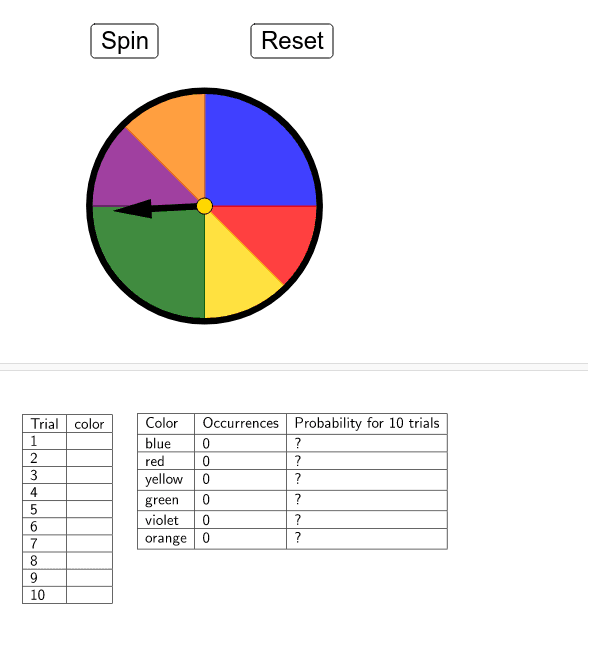
This example demonstrates probability through experimental simulations, visually showing the relationship between the frequency of random events and theoretical probability. It involves core concepts like probability & statistics, frequency distribution, sample space, and events. GeoGebra commands and objects used include CountIf, Circle, Rotate, Vector, Line, OrthogonalLine, Intersect, CircleSector, Midpoint, IsInRegion, Sum, Element, TableText, and FractionText. Suitable for high school probability & statistics education to understand the connection between experimental and theoretical probabilities and data processing methods.
GeoGebra Commands & Parameters
CountIf(x ≟ "orange", B2:B11) → E7CountIf(x ≟ "violet", B2:B11) → E6CountIf(x ≟ "green", B2:B11) → E5CountIf(x ≟ "yellow", B2:B11) → E4CountIf(x ≟ "red", B2:B11) → E3CountIf(x ≟ "blue", B2:B11) → E2Circle(A, B) → cRotate(S0, ((-a))°, A) → CVector(A, C) → uLine(B, A) → bOrthogonalLine(A, b) → eIntersect(c, e) → D, ECircleSector(A, E, B) → fIntersect(c, b) → F, GMidpoint(G, E) → HLine(A, H) → gIntersect(c, g) → I, JCircleSector(A, J, E) → hCircleSector(A, G, J) → kCircleSector(A, D, G) → pCircleSector(A, I, D) → qCircleSector(A, B, I) → rIsInRegion(C, f) → iIsInRegion(C, h) → jSum(Sequence[(IsInRegion[C, Element[liste2, k]] * k), k, 1, 6]) → mElement(liste1, m) → texte1TableText({{A1, B1}, {A2, B2}, {A3, B3}, {A4, B4}, {A5, B5}, {A6, B6}, {A7, B7}, {A8, B8}, {A9, B9}, {A10, B10}, {A11, B11}}, "|_") → text1FractionText(F2) → F_22FractionText(F3) → F_32FractionText(F4) → F_42FractionText(F5) → F_52FractionText(F6) → F_62FractionText(F7) → F_72TableText({{D1, E1, F1}, {D2, E2, F_22}, {D3, E3, F_32}, {D4, E4, F_42}, {D5, E5, F_52}, {D6, E6, F_62}, {D7, E7, F_72}}, "|_") → text2