
Experimental Probability by tmoorehead
Loading the math board and drawing, please wait…
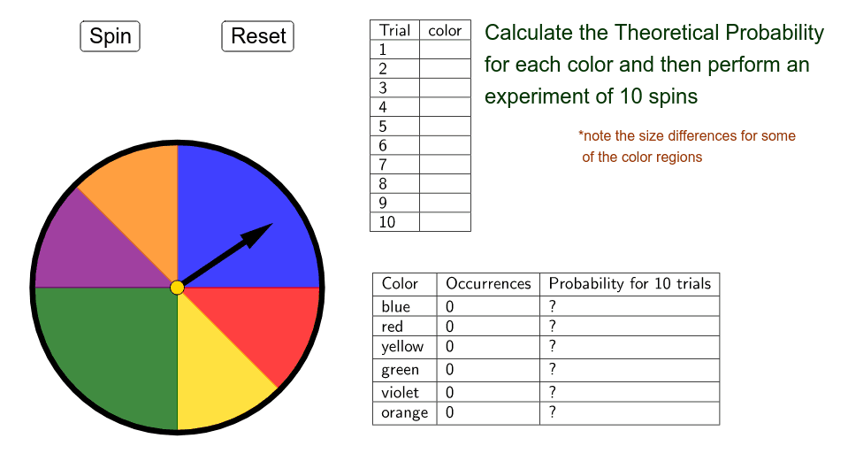
This example demonstrates experimental probability in probability & statistics through simulations. Core concepts include probability, random variables, and histograms. It utilizes GeoGebra commands like CountIf, Circle, Rotate, Vector, Line, OrthogonalLine, Intersect, CircleSector, Midpoint, IsInRegion, Sum, Element, and TableText. Suitable for high school students learning probability theory and understanding the difference between theoretical and experimental probability.
GeoGebra Commands & Parameters
CountIf(x ≟ "orange", B2:B11) → E7CountIf(x ≟ "violet", B2:B11) → E6CountIf(x ≟ "green", B2:B11) → E5CountIf(x ≟ "yellow", B2:B11) → E4CountIf(x ≟ "red", B2:B11) → E3CountIf(x ≟ "blue", B2:B11) → E2Circle(A, B) → cRotate(S0, ((-a))°, A) → CVector(A, C) → uLine(B, A) → bOrthogonalLine(A, b) → eIntersect(c, e) → D, ECircleSector(A, E, B) → fIntersect(c, b) → F, GMidpoint(G, E) → HLine(A, H) → gIntersect(c, g) → I, JCircleSector(A, J, E) → hCircleSector(A, G, J) → kCircleSector(A, D, G) → pCircleSector(A, I, D) → qCircleSector(A, B, I) → rIsInRegion(C, f) → iIsInRegion(C, h) → jSum(Sequence[(IsInRegion[C, Element[liste2, k]] * k), k, 1, 6]) → mElement(liste1, m) → texte1TableText({{A1, B1}, {A2, B2}, {A3, B3}, {A4, B4}, {A5, B5}, {A6, B6}, {A7, B7}, {A8, B8}, {A9, B9}, {A10, B10}, {A11, B11}}, "|_") → text1TableText({{D1, E1, F1}, {D2, E2, F2}, {D3, E3, F3}, {D4, E4, F4}, {D5, E5, F5}, {D6, E6, F6}, {D7, E7, F7}}, "|_") → text2