
Expected Value & Root Statistical Visualization
Loading the math board and drawing, please wait…
In collections
Mapping Diagrams: From AB to C&DE, Resource
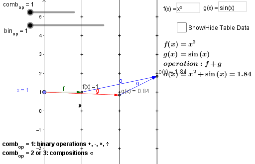
This example demonstrates how to visualize the statistical relationship between expected value and roots using histograms and scatter plots in GeoGebra. Key math concepts include expected value calculation, root finding, and data distribution analysis. Construction highlights involve commands like Element, Point, Vector, Sequence, Zip, Textfield, and objects such as ops, bin_{op}, op, comb_{op} for data processing. Suitable for high school and above learners to understand the integration of statistics and geometry.
GeoGebra Commands & Parameters
Element(ops, bin_{op}) → opPoint(yAxis) → AElement(fnlist, comb_{op}) → oVector(A, B) → uVector(A, C) → vVector(B, D) → wVector(C, D) → aVector(A, B) → bVector(B, E) → cVector(A, F) → dVector(F, E) → eVector(B, E) → hSequence(-5, 5) → list1Zip((a1, b), b, list1) → list2Zip((a2, b), b, list1) → list3Zip((a3, b), b, list1) → list4Textfield(f) → InputBox1Textfield(g) → InputBox2Zip((s, t), s, lista, t, listo) → list5Zip((0, s), s, lista) → list6Zip((a3, s), s, listo) → list7Zip(Vector[S, T], S, list6, T, list7) → list8Zip((a2, s), s, listo) → list9Zip(Vector[S, T], S, list6, T, list9) → list10
AI Drawing Prompt Reference
Create a visualization showing the statistical relationship between expected value and roots using histograms and scatter plots. Start by generating a data sequence, then create multiple vectors by connecting key points to form geometric structures. Draw vectors based on input values and use these to generate several lists. Finally, plot these lists as histograms and scatter plots to illustrate the data relationships.
The prompt above was compiled from the original drawing commands and is for reference only.