
Expanding and Reducing Fractions by Anthony OR 柯志明
Loading the math board and drawing, please wait…
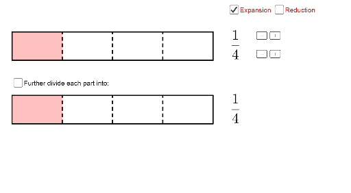
This example demonstrates the process of expanding and reducing fractions, illustrating key mathematical concepts such as the fundamental properties of fractions, methods of simplification and expansion, greatest common divisors, and least common multiples. It utilizes GeoGebra commands like Sequence, If, Element, Point, Polygon, Textfield, and Corner to dynamically visualize fraction operations. Suitable for middle school and above, it helps learners understand the geometric and algebraic principles behind fraction arithmetic.
GeoGebra Commands & Parameters
Sequence(B + ((i * l / q), w), i, 1, p) → list3If(q > 9 ∨ p > 9, true, false) → digit2If(digit2, (9.1, -2.75), (8, -2.75)) → Q2If(digit2, (6.8, -2.75), (6, -2.75)) → Q1If(digit2, (9.1, -1.6), (8, -1.6)) → P2If(digit2, (6.8, -1.6), (6, -1.6)) → P1Element(list3, u) → PSequence(B + (i * (x(P) - x(B), 0)), i, 1, floor(l / (x(P) - x(B)))) → list4Point(list4) → P'Polygon(B, B + (l, 0), B + (l, w), B + (0, w)) → poly2, a_2, b_2, c_2, d_2Polygon(A, A + (l, 0), A + (l, w), A + (0, w)) → poly1, a_1, b_1, c_1, d_1Sequence(Segment[A + ((i * l / q), 0), A + ((i * l / q), w)], i, 1, q - 1) → list1Polygon(A, A + ((p * l / q), 0), A + ((p * l / q), w), A + (0, w)) → poly3, a, b, c, dPolygon(B, B + ((p * l / q), 0), B + ((p * l / q), w), B + (0, w)) → poly4, e, f, m, nSequence(Segment[B + ((i * l / q), 0), B + ((i * l / q), w)], i, 1, q - 1) → list2Textfield(p) → inputBox1Textfield(q) → inputBox2Sequence(Polygon[B + (i * (x(P) - x(B), 0)), B + ((i * (x(P) - x(B))), w), B + (((i - 1) * (x(P) - x(B))), w), B + ((i - 1) * (x(P) - x(B), 0))], i, 1, (x(P') - x(B)) / (x(P) - x(B))) → list5Sequence(Segment[A + ((i * l / q), 0), A + ((i * l / q), w)], i, 1, q - 1) → list1_1Sequence(Segment[B + ((i * l / q), 0), B + ((i * l / q), w)], i, 1, q - 1) → list2_1Sequence(Sequence[Segment[B + ((i * l / q) + (j * l / ((q * r))), 0), B + ((i * l / q) + (j * l / ((q * r))), w)], i, 0, q - 1], j, 1, r - 1) → list6Textfield(input1) → InputBox1Textfield(input2) → InputBox2If(ans1 ≟ (r * p), true, false) → correct1If(ans2 ≟ (r * q), true, false) → correct2Polygon(P1, P1 + (1.3, 0), P1 + (1.3, -1), P1 + (0, -1)) → poly5, f_1, g_1, h_1, i_1Polygon(Q1, Q1 + (1.3, 0), Q1 + (1.3, -1), Q1 + (0, -1)) → poly6, j_1, k_1, l_1, m_1Polygon(Q2, Q2 + (1.3, 0), Q2 + (1.3, -1), Q2 + (0, -1)) → poly8, s_1, t_1, e_1, f_2Polygon(P2, P2 + (1.3, 0), P2 + (1.3, -1), P2 + (0, -1)) → poly7, n_1, p_1, q_1, r_1Corner(text1, 3) → EIf(Length[list4] ≠ 1 ∧ IndexOf[P', list4] ≠ Length[list4], true, false) → arrowSequence(Segment[B + (i * (x(P) - x(B), 0)), B + ((i * (x(P) - x(B))), w)], i, 1, (x(P') - x(B)) / (x(P) - x(B)) - 1) → list7Textfield(input3) → InputBox3Textfield(input4) → InputBox4If(ans4 ≟ q / div, true, false) → correct4If(ans3 ≟ p / div, true, false) → correct3If(digit2, (6.7, -2.1), (5.9, -2.1)) → HIf(digit2, (8.6, -2.1), (7.8, -2.1)) → IIf(digit2, (6.7, -3.4), (5.9, -3.4)) → JIf(digit2, (8.6, -3.4), (7.8, -3.4)) → KPolygon(H, H + (1.3, 0), H + (1.3, -1), H + (0, -1)) → poly9, h_2, j, k, g_2Polygon(J, J + (1.3, 0), J + (1.3, -1), J + (0, -1)) → poly10, j_2, i_2, k_2, l_2Polygon(I, I + (1.3, 0), I + (1.3, -1), I + (0, -1)) → poly11, i_3, m_2, n_2, p_2Polygon(K, K + (1.3, 0), K + (1.3, -1), K + (0, -1)) → poly12, k_3, q_2, r_2, s_2
AI Drawing Prompt Reference
Create a dynamic visualization showing the expansion and reduction of fractions. Include two rectangles that dynamically divide and combine to illustrate fraction operations. The diagram should show the numerator and denominator of fractions and demonstrate fraction expansion and reduction through area changes in the rectangles. Key elements are two rectangles, multiple line segments, points, and text boxes for input and display. Start by drawing two rectangles, then dynamically divide them based on input fractions, and finally show the fraction operations through area changes.
The prompt above was compiled from the original drawing commands and is for reference only.