
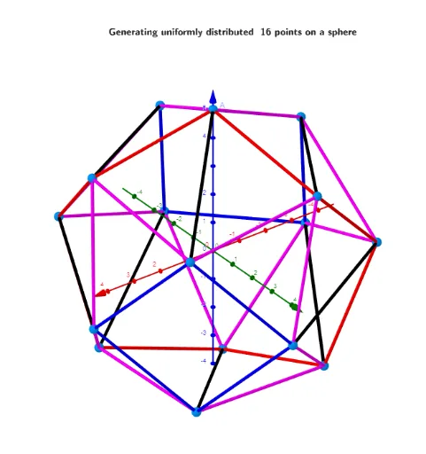
Example of Non-uniqueness of Extreme Distribution for n=16 Particles on a Sphere
Loading the math board and drawing, please wait…
① This example demonstrates that for 16 particles placed on the surface of a sphere, the extreme distribution (e.g., minimizing potential energy or maximizing symmetry) is not unique, with multiple equivalent configurations existing. ② Core mathematical concepts include spherical geometry, combinatorial optimization, extreme distributions, symmetry, non-uniqueness, and balanced arrangement of points on a curved surface. ③ Construction highlights: The GeoGebra commands used include Sphere to create the sphere, PointIn to generate particles on the surface, Sequence and Zip for batch processing coordinates, Textfield and InputBox for interactive parameter input, TableText for data display, and buttons to control calculations. Key objects include spheres, points, texts, sliders, and input boxes. ④ This is suitable for high school to university-level teaching in mathematics or physics, useful for exploring spherical point distribution problems, optimization algorithms, and geometric symmetry, and can serve as a demonstration for mathematical modeling or computational geometry.
GeoGebra Commands & Parameters
Sphere((0, 0, 0), R) → d_1Textfield(n) → InputBox2Textfield(h) → InputBox3Textfield(R) → InputBox1PointIn(d_1) → AAppend(A, Sequence[((random(), random(), random()) * R), i, 2, n]) → l2sTableText({Join[{{"n"}, Sequence[i, i, 4, 57 + 3]}], Join[{{" p_n=P_n/[R*n*(n-1)/2]"}, l1}]}, "vl") → text8Textfield(i) → InputBox5Textfield(Um002) → InputBox4Sequence(Sequence[Segment[Element[R01'_1, k], Element[R01'_1, t]], t, k + 1, n], k, 1, n - 1) → segments1UnicodeToLetter(34) → u34Text("\;\;\;\;\;\;\;\;\;\;\;\;\;\bgcolor{#F2F3F4}{\fgcolor{" + (If[cc1', "orange", "#536872"]) + "} \boxed{ " + cc1' + ("}}\;\;\;\; \;\;\;\;\; \\ \;\; ( accuracy- up\; to\;\; 2*10^{" - k_2) + ("\;})\;\\\;\; ➤➤➤\;\;\;\scalebox{1.3}{ " + (ScientificText[cc1, 3])) + "}\;█ ", B01, true, true) → text01Text("\;\;\;\;\;\;\;\;\;\;\;\;\;\bgcolor{#F2F3F4}{\fgcolor{" + (If[cc2', "orange", "#536872"]) + "} \boxed{ " + cc2' + ("}}\;\;\;\; \;\;\;\;\; \\ \;\; ( accuracy- up\; to\;\; 2*10^{" - k_2) + ("\;})\;\\\;\; ➤➤➤\;\;\;\scalebox{1.3}{ " + (ScientificText[cc2, 3])) + "}\;█ ", B02, true, true) → text02Sequence(Sequence[Segment[Element[R01'_2, k], Element[R01'_2, t]], t, k + 1, n], k, 1, n - 1) → segments2Sum(Flatten[Sequence[Append[Sequence[Element[Um1, i], i, m101(k), m201(k)], " "], k, 1, 5]]) → txtUm11ptxt(Text[Sum11]) → txtsum11ptxt(Text[Sum12]) → txtsum12ptxt(Text[Sum21]) → txtsum21ptxt(Text[Sum22]) → txtsum22ptxt(Text[Element[l1, n - 3]]) → txttableTableText(lp00, lp11, lp22, "v") → text6dZip(Segment[Element[R01'_1, y(a)], Element[R01'_1, z(a)]], a, lr_1b(1)) → ll_11Zip(Segment[Element[R01'_1, y(a)], Element[R01'_1, z(a)]], a, lr_1b(2)) → ll_12Zip(Segment[Element[R01'_1, y(a)], Element[R01'_1, z(a)]], a, lr_1b(3)) → ll_13Zip(Segment[Element[R01'_1, y(a)], Element[R01'_1, z(a)]], a, lr_1b(4)) → ll_14Zip(Length[a], a, {ll_11, ll_12, ll_13, ll_14}) → lä_1Zip(Segment[Element[R01'_2, y(a)], Element[R01'_2, z(a)]], a, lr_2b(1)) → ll_21Zip(Segment[Element[R01'_2, y(a)], Element[R01'_2, z(a)]], a, lr_2b(2)) → ll_22Zip(Segment[Element[R01'_2, y(a)], Element[R01'_2, z(a)]], a, lr_2b(3)) → ll_23Zip(Segment[Element[R01'_2, y(a)], Element[R01'_2, z(a)]], a, lr_2b(4)) → ll_24Zip(Length[a], a, {ll_21, ll_22, ll_23, ll_24}) → lä_2
AI Drawing Prompt Reference
In a 3D scene, place a sphere as the main geometric object, with user inputs for the particle count n, a height parameter h, and the sphere radius R. Generate n points randomly on the sphere’s surface to represent particles. Display a related normalized quantity depending on n in a table-like text area. Then construct and draw multiple groups of short line segments that illustrate the structured connections between corresponding points, using an indexed sequence so the segment sets appear in parallel. Add on-screen text elements to present the extreme-distribution discussion and accuracy-related numeric items, and include controls that let the viewer trigger the displayed computations.
The prompt above was compiled from the original drawing commands and is for reference only.