
Euler's Theorem: Multiple Geometric Demonstrations (Triangle, Circles, and Const
Loading the math board and drawing, please wait…
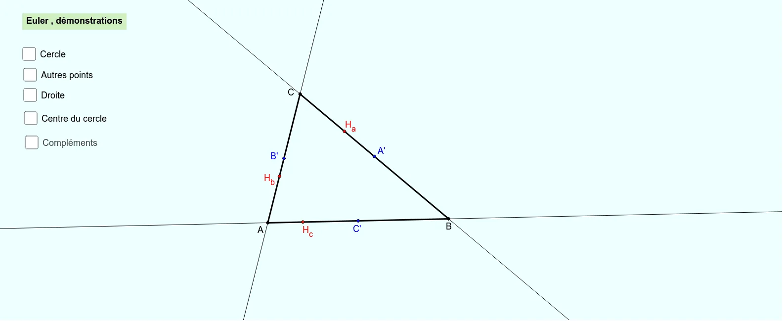
This GeoGebra example, titled 'Euler (démonstrations)', provides a comprehensive dynamic visualization of Euler's theorem in triangle geometry. It demonstrates the collinearity of the centroid, circumcenter, orthocenter, and the nine-point center (Euler line), along with the construction of related circles such as the circumcircle, incircle, and excircles. The construction involves core mathematical concepts including triangle centers, perpendicular bisectors, angle bisectors, medians, altitudes, and circle properties. Using GeoGebra commands such as Line, OrthogonalLine, CircumcircleArc, Segment, Intersect, Circle, Angle, Polygon, Midpoint, Ray, LineBisector, and AngularBisector, the example builds multiple objects (points A, B, C, H, O, etc.) and auxiliary circles/polygons to illustrate the relationships. It is suitable for high school and university students or teachers exploring classical geometry theorems, and serves as an advanced exercise in dynamic geometric construction and theorem verification.
GeoGebra Commands & Parameters
Line(A, B) → aLine(B, C) → bLine(C, A) → cOrthogonalLine(C, a) → dC_Euler(A, B, C) → D_1, e, B', A', C'Point(e) → FPoint(e) → G_1CircumcircleArc(G_1, A', F) → gSegment(C', A') → hSegment(B', C) → iSegment(B', A) → jIntersect(a, d) → H_cSegment(H_c, B') → kCircle(B', H_c) → pAngle(C, H_c, A) → αPolygon(B', A', C', H_c) → poly1, b', a', c', h_cOrthogonalLine(B, c) → nIntersect(d, n) → HMidpoint(H, C) → H_3Polygon(A, H, C) → poly2, c_1, a_1, h_1Ray(B', H_3) → qIntersect(b, q) → I_1Ray(H_3, A') → rRay(H_3, C') → sSegment(C', B') → tAngle(C', B', H_3) → βPoint(e) → JPoint(e) → KCircumcircleArc(J, H_c, K) → d_1Ray(A, H) → b_1Intersect(b, b_1) → LAngle(C, L, A) → γCercle_3pts(A, C, B) → O, e_1Line(A, O) → f_1Intersect(e_1, f_1, 2) → DSegment(C, D) → g_1Segment(D, B) → i_1Angle(A, C, D) → δAngle(D, B, A) → εOrthogonalLine(B, c) → j_1Polygon(B, H, C, D) → poly3, b_2, h_2, c_2, d_2Segment(H, D) → k_1Segment(A, A') → l_1TriPart(A, A') → G, MPolygon(A, H, D) → poly4, d_3, a_2, h_3Segment(H, O) → m_1Polygon(C, H, O, C') → poly5, c_3, h_4, o, c'_1OrthogonalLine(A, b) → n_1OrthogonalLine(B, h_1) → p_1Intersect(c, p_1) → H_bIntersect(b, n_1) → H_aLineBisector(H_c, C') → q_1Segment(H, O) → r_1Segment(O, C') → s_1Segment(O, A') → t_1Segment(O, B') → e_2Segment(H, H_c) → f_2Segment(H, H_b) → g_2Segment(H, H_a) → i_2LineBisector(H_a, A') → j_2LineBisector(H_b, B') → k_2Intersect(d_1, b_1) → H_1, QMidpoint(H, B) → H_2C_Inscrit(A, C, B) → I, p_2AngularBisector(h_1, b) → l_2, m_2AngularBisector(b, a) → n_2, q_2Intersect(l_2, q_2) → EIntersect(l_2, n_2) → NIntersect(m_2, n_2) → POrthogonalLine(P, a) → r_2OrthogonalLine(N, b) → s_2OrthogonalLine(E, h_1) → t_2Intersect(a, r_2) → RIntersect(s_2, b) → SIntersect(t_2, c) → TCircle(N, S) → e_3Circle(P, R) → f_3Circle(E, T) → g_3Intersect(e, g_3) → F_2, , ,Intersect(e, e_3) → F_1, , ,Intersect(e, f_3) → F_3, , ,Intersect(e, p_2) → F_e, , ,Intersect(g_3, b, 2) → UIntersect(g_3, a, 2) → VIntersect(f_3, b, 1) → A_1Intersect(e_3, a, 1) → B_1Intersect(e_3, c, 2) → WIntersect(f_3, c, 1) → ZSegment(A, B) → a_3Segment(B, C) → b_3Segment(C, A) → i_3
AI Drawing Prompt Reference
Draw a triangle with its three side lines extended. From one vertex, drop a perpendicular to the opposite side, marking the foot. Construct the circumcircle of the triangle and label its center. Draw segments from the orthocenter to a point on the circumcircle)Skip that; instead, connect the orthocenter to the triangle's vertices and the circumcenter. Construct a midline of the triangle and mark its midpoint. Inside the triangle, form a polygon using the orthocenter, circumcenter, and a vertex. Then draw a ray from a vertex intersecting the opposite side. Finally, label several key angles and add auxiliary circles tangent to the triangle's sides.
The prompt above was compiled from the original drawing commands and is for reference only.