
Error Difference of Pi at a=5000
Loading the math board and drawing, please wait…
In collections
Complex Math
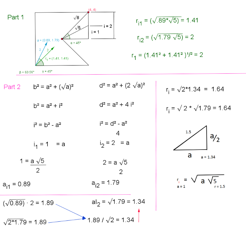
This example demonstrates the error difference of Pi when a=5000. It involves the geometric construction and error analysis of Pi. Using GeoGebra commands such as semicircle, segment, circle, polygon, vector, etc., a geometric model is constructed to illustrate the error difference. Suitable for high school mathematics education and learning.
GeoGebra Commands & Parameters
Semicircle(C, D) → cSemicircle(D, C) → dSegment(A, D) → aCircle(A, 1) → fSemicircle(E, F) → rSemicircle(F, E) → gPolygon(B, A, C, G) → poly1, b_1, a_1, c_1, g_1Vector((1.414213562373095, 1.414213562373095)) → u_3Vector((1.79, 0.89)) → vSegment(G, B) → eSegment(G, J) → hSegment(G, K) → iAngle(B, G, K) → α_uAngle(B, G, J) → β_vVector((0.89, 1.79)) → wSegment(G, L) → jAngle(B, G, L) → δ_wAngle(J, G, L) → Δ_vCircle(G, K) → kPoint(r) → NPoint(g) → MSegment(N, A) → pSegment(A, M) → qSegment(M, N) → sPolygon(N, C, G, B, M) → poly2, n_1, c_2, g_2, b_2, m_1Vector((2, 1)) → tVector((1, 2)) → uSegment(G, N) → d_1Segment(G, M) → e_1Angle(M, G, N) → α_tSegment(A, R) → k_1Segment(A, Q) → l_1Segment(Q, R) → p_1Circle(A, S) → q_1Distance(G, A) → distanceGAPoint(Circle[A, 3]) → TSegment(A, T) → r_1Point(Circle[G, 3]) → USegment(G, U) → s_1Point(Circle[T, 2.8284271247461903]) → VSegment(T, V) → t_1Distance(G, Q) → distanceGQDistance(G, M) → distanceGMSegment(G, M) → a_2Segment(W, Z) → d_2Vector(A_1, B_1) → u_2Vector(C_1, D_1) → v_2Distance(G, N) → distanceGNSegment(G, N) → f_2Distance(G, Q) → j_2Point(k) → E_1Point(k) → F_1Distance(F_1, E_1) → distanceF1E1Segment(E_1, F_1) → k_2Point(k_2) → G_1Point(s) → H_1Distance(G_1, H_1) → distanceG1H1Segment(G_1, H_1) → l_2Segment(I_1, J_1) → m_2Segment(K_1, L_1) → n_2Segment(K_2, L_2) → n_3Segment(K_3, L_3) → n_4Segment(K_4, L_4) → n_5Segment(K_5, L_5) → n_6Segment(K_8, L_8) → n_9Polygon(M_1, N_1, O_1, P_1) → poly3, m_3, n_{13}, o_2, p_2Intersect(k, q_1, 1) → Q_1Point(f_2) → R_1Circle(Q_1, R_1) → q_2Mirror(q_2, i) → r_2Segment(S_1, T_1) → a_3Segment(U_1, V_1) → b_3Intersect(f_3, i, 1) → W_1Point(f_3) → Z_1Segment(W_1, Z_1) → d_3Textfield(σ) → inputBox1Point(f_3) → C_2Point(f_3) → D_2Vector(G, D_2) → v_3Distance(G, D_2) → distanceGD2Vector(E_2, F_2) → w_3Mirror(N, p_1) → N'Mirror(A, p_1) → A'Segment(N', A') → p'Mirror(A, p_1) → A'_1Mirror(R, p_1) → R'Segment(A'_1, R') → g_3Mirror(A, p_1) → A'_2Mirror(M, p_1) → M'Segment(A'_2, M') → q'Mirror(A, p_1) → A'_3Mirror(Q, p_1) → Q'Segment(A'_3, Q') → h_3Segment(G, D_2) → i_3Slope(i_3) → m_4Point(p_3) → G_2Distance(G, G_2) → distanceGG2Vector(G, G_2) → j_3Segment(G, G_2) → l_3Angle(K, G, G_2) → αPoint(q_3) → H_2Point(s_3) → I_2Point(r_3) → J_2Polygon(H_2, I_2, J_2, G) → poly4, h_4, i_4, j_4, g_4Point(h_4) → M_2Point(j_4) → N_2Point(i_4) → O_2Point(g_4) → P_2Segment(O_2, M_2) → t_3Segment(N_2, P_2) → a_4Point(a_4) → Q_2Point(t_3) → R_2Segment(Q_2, R_2) → b_4Point(i_4) → T_2Point(f_4) → U_2Point(e_4) → S_2Segment(S_2, U_2) → k_4Point(p_4) → V_2Segment(G, V_2) → l_4Point(Circle[E_1, 1.35]) → W_2Segment(E_1, W_2) → q_4Polygon(B_3, C_3, D_3, E_3) → poly5, b_5, c_5, d_5, e_5Polygon(F_3, G_3, H_3, I_3) → poly6, f_5, g_5, h_5, i_5Polygon(J_3, M_3, N_3, O_3) → poly7, j_5, m_5, n_7, o_5Segment(R_3, S_3) → a_5Intersect(f, p, 1) → T_3Point(f) → U_3Semicircle(T_3, U_3) → k_5Mirror(A, p) → A'_4Mirror(M, p) → M'_1Mirror(A, k_1) → A'_5Mirror(Q, k_1) → Q'_1Segment(A'_5, Q'_1) → l_5Segment(V_3, W_3) → p_5Segment(R_4, S_4) → a_6Segment(V_4, W_4) → p_6
AI Drawing Prompt Reference
Draw a unit circle f centered at point A, and a segment e with endpoints G and A. Then construct a circle k centered at G with radius sqrt(2), and find its intersection points N and M with circle f. Connect points N and A, M and A, and N and M to form a triangle. Finally, draw vector u from G to A and vector d from G to N to show the relationship between the vectors.
The prompt above was compiled from the original drawing commands and is for reference only.