
Dynamic Illustration of Incircle and Excircle Collinearity in Right Triangles
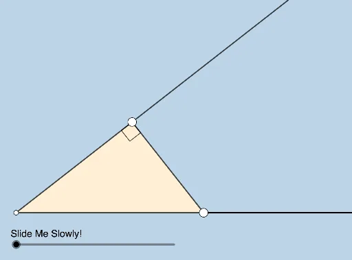
Loading the math board and drawing, please wait…
This example dynamically illustrates the collinearity of the incircle and excircles of a right triangle. It involves core mathematical concepts such as incircle, excircle, properties of right triangles, and trigonometric functions. The construction utilizes GeoGebra commands like Intersect, Semicircle, Point, Polygon, Angle, Rotate, Ray, Segment, Circle, OrthogonalLine, Min, Dilate, and CircleSector. Suitable for high school mathematics education to understand special geometric properties and dynamic geometric transformations.
GeoGebra Commands & Parameters
Intersect(xAxis, yAxis) → ASemicircle(A, B) → cPoint(c) → CPolygon(A, C, B) → t1, b, a_1, c_1Angle(B, A, C) → αRotate(B, α / 2, A) → B'Angle(B, A, B') → βRay(A, B') → fRotate(A, π / 4, C) → A'Ray(C, A') → gRay(A, C) → hRay(A, B) → iSegment(B, C) → jIntersect(g, f) → DRay(B, B + (1, 0, 0)) → kPoint(k) → ECircle(C, 3) → dIntersect(d, h, 2) → FAngle(E, B, C, xOyPlane) → γRotate(E, γ / 2, B) → E'Ray(B, E') → lRotate(B, π / 4, C) → B'_1Ray(C, B'_1) → mIntersect(l, m) → GOrthogonalLine(D, h) → nOrthogonalLine(D, k, xOyPlane) → pIntersect(n, h) → HIntersect(p, i) → IOrthogonalLine(G, h, xOyPlane) → qOrthogonalLine(G, k, xOyPlane) → rIntersect(q, h) → JIntersect(r, i) → KCircle(G, J, xOyPlane) → eCircle(D, H) → sRay(B, D) → tAngle(A, C, B) → δRay(B, D) → f_1Ray(A, D) → g_1Min({Distance[A, D], Distance[B, D], Distance[B, G], Distance[C, G]}) → oCircle(A, (0.35 * o)) → d_1Intersect(d_1, i) → L,Circle(B, (0.35 * o)) → e_1Circle(C, (0.35 * o)) → h_1Intersect(h_1, h, 2) → MIntersect(k, e_1) → N,Intersect(e_1, j) → O,Dilate(A, If[0 < u ≤ 1, 1 - u, 0], D) → A'_1Segment(A, A'_1) → i_1Dilate(B, If[0 < u ≤ 1, 1 - u, 0], D) → B'_2Segment(B, B'_2) → j_1Rotate(O, If[0 < u ≤ 1, (u * (π / 2 - α) / 2), (π / 2 - α) / 2], B) → O'Rotate(L, If[0 < u ≤ 1, (u * β), β], A) → L'CircleSector(B, O, O') → k_1CircleSector(A, L, L') → p_1Dilate(C, If[1 < u ≤ 2, 2 - u, 0], G) → C'Dilate(B, If[1 < u ≤ 2, 2 - u, 0], G) → B'_3Segment(B, B'_3) → l_1Segment(C, C') → m_1Intersect(h_1, j) → P,Rotate(P, If[1 < u ≤ 2, ((u - 1) * π / 4), π / 4], C) → P'Rotate(N, If[1 < u ≤ 2, ((u - 1) * γ / 2), γ / 2], B) → N'CircleSector(B, N, N', xOyPlane) → q_1CircleSector(C, P, P') → r_1Rotate(p_1, If[2.5 < u ≤ 3.5, ((u - 2.5) * β), β], A) → s_1Rotate(k_1, If[2.5 < u ≤ 3.5, ((u - 2.5) * (π / 2 - α) / 2), (π / 2 - α) / 2], B) → t_1Rotate(q_1, If[3.5 < u ≤ 4.5, ((u - 3.5) * γ / 2), γ / 2], B) → c_2Rotate(r_1, If[3.5 < u ≤ 4.5, ((u - 3.5) * π / 4), π / 4], C) → d_2Dilate(D, If[5 < u ≤ 6, 6 - u, 0], H) → D'Circle(D, D') → e_2OrthogonalLine(D, j) → n_1Intersect(j, n_1) → QDilate(G, If[6 < u ≤ 7, 7 - u, 0], J) → G'Circle(G, G', xOyPlane) → f_2OrthogonalLine(G, j, xOyPlane) → b_1Intersect(b_1, j) → RDilate(H, If[12 < u ≤ 13, 13 - u, 0], R) → H'Segment(H, H') → g_2Dilate(R, If[13 < u ≤ 14, 14 - u, 0], K) → R'Segment(R, R') → h_2
AI Drawing Prompt Reference
Illustrate the collinearity of the incircle and excircles in a right triangle dynamically. Start with the intersection of coordinate axes, draw a semicircle with the hypotenuse as diameter to form the triangle. Rotate the right angle vertex by half its angle to find a point, then draw rays. Rotate the vertex by 45 degrees to draw another ray. The intersection points help determine the excircle and incircle. Add auxiliary lines and circles to show their collinearity, suitable for high school geometry education.
The prompt above was compiled from the original drawing commands and is for reference only.