
Dynamic Graphing Solution of Systems of Linear Inequalities
Loading the math board and drawing, please wait…
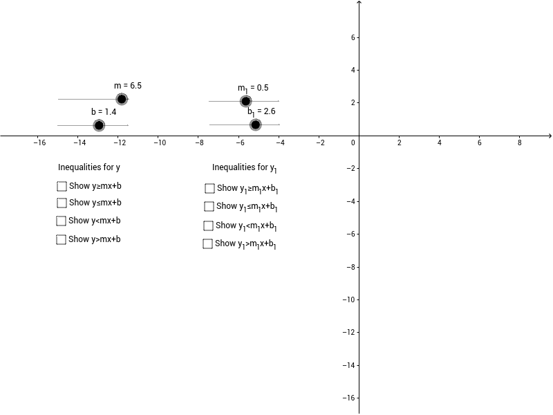
This GeoGebra applet demonstrates the graphical solution of systems of linear inequalities using slope and y-intercept parameters. The core mathematical concepts include linear functions, half-plane inequalities, intersection of solution regions, and the geometric interpretation of feasible sets. Constructed from objects such as m, b, a, c, m_1, b_1 and auxiliary points j, k, l, n, o, p, q, r, the example uses GeoGebra commands to define boundary lines, input inequalities, shade feasible regions, and label key elements with text1 and text2. It is suitable for middle school algebra (grades 7–9) and high school coordinate geometry review, supporting interactive classroom demonstrations and student exploration of inequality systems.
GeoGebra Commands & Parameters
Numeric m(-2.7)Numeric b(1.4)y ≥ m * x + by ≤ m * x + bNumeric m_1(0.5)Numeric b_1(2.6)Boolean d(false)Boolean e(false)y ≥ m_1 * x + b_1Boolean g(false)y ≤ m_1 * x + b_1Boolean i(false)y < m * x + bBoolean k(false)y > m * x + bBoolean n(false)y < m_1 * x + b_1Boolean p(false)y > m_1 * x + b_1Boolean r(false)
AI Drawing Prompt Reference
Draw a graph of a system of inequalities with two lines. Set the slope of the first line to -2.7 and the y-intercept to 1.4, and draw the boundary lines y ≥ -2.7x + 1.4 and y ≤ -2.7x + 1.4. Set the slope of the second line to 0.5 and the y-intercept to 2.6, and draw the boundary lines y ≥ 0.5x + 2.6 and y ≤ 0.5x + 2.6. Color the feasible regions according to the selections and label key points with text.
The prompt above was compiled from the original drawing commands and is for reference only.