Dynamic Demonstration of Trigonometric Functions and Differential Equations on a

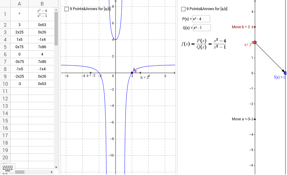
This GeoGebra example constructs a 3D cylindrical surface and dynamically displays the relationship among trigonometric functions, hyperbolic functions, and solutions of differential equations on it. Core mathematical concepts include parametric equations of a cylinder, sine and hyperbolic functions, solution curves of differential equations, and visualization of vector fields and point sequences. Construction highlights: commands such as Point, Vector, Textfield, and Sequence are used to create point lists, vectors, and input boxes; objects like A, B, C define the cylinder parameters; list1 and list2 store point sequences, while show_{points/arrows} toggles the visibility of points and arrows; input boxes inputBox1 and inputBox2 allow users to adjust parameters in real time, updating the curve shapes. Suitable for high school to undergraduate mathematics education, this example helps students intuitively understand function curves on curved surfaces, spatial forms of differential equation solutions, and parametric dynamic interaction.