
Dynamic Demonstration of Step Functions
Loading the math board and drawing, please wait…
In collections
Complex Math
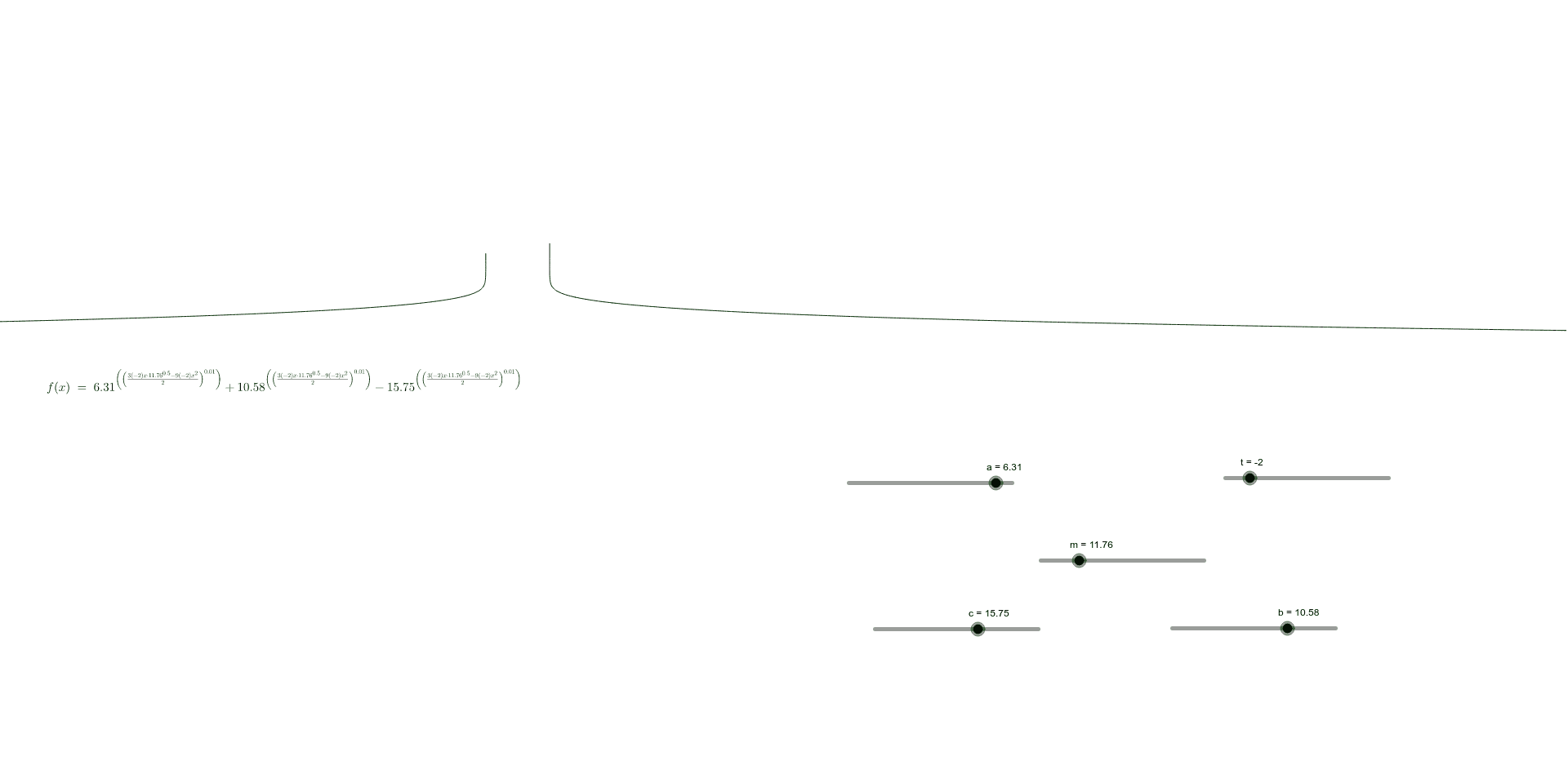
This example provides an interactive visualization of a step function, highlighting its characteristic discontinuous behavior. The demonstration focuses on core mathematical concepts such as piecewise functions, limits, and jump discontinuities. The construction utilizes GeoGebra objects including parameters (a, t, m, n, b, c) to control the intervals and constant values of the segments, culminating in the definition of the function f. This tool is ideal for high school students or undergraduate calculus learners to explore the properties of piecewise constant functions and the concept of discontinuity.
GeoGebra Commands & Parameters
Numeric a(6.3100000000000005)Numeric t(-2.0)Numeric m(11.7577)Numeric n(0.01002)Numeric b(10.577950000000001)Numeric c(15.75407)f(x) = a^((((((3 * t) * x) * m^(0.5)) - ((9 * t) * x^(2))) / 2)^(n)) + b^((((((3 * t) * x) * m^(0.5)) - ((9 * t) * x^(2))) / 2)^(n)) - c^((((((3 * t) * x) * m^(0.5)) - ((9 * t) * x^(2))) / 2)^(n))
AI Drawing Prompt Reference
Draw a dynamic demonstration of a step function with parameters a, t, m, n, b, and c to control intervals and constant values, showcasing its discontinuous behavior, particularly the characteristics of step functions, piecewise functions, limits, and jump discontinuities.
The prompt above was compiled from the original drawing commands and is for reference only.