Dynamic Demonstration of Binomial Confidence Intervals and Histogram

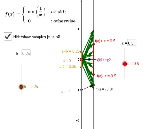
This GeoGebra example interactively demonstrates the relationship between confidence intervals, limits, and histograms in the context of a binomial distribution. Core mathematical concepts include binomial distribution, confidence intervals, sample proportion estimation, and the limiting behavior as sample size increases. The construction uses commands such as Point, Vector, Textfield, Segment, Line, Derivative, Intersect, Polygon, and Sequence to build coordinate axes, reference lines, and histogram bars. Input boxes allow users to adjust parameters, while a button triggers dynamic updates. Suitable for high school to university statistics and probability courses, it helps learners visualize how confidence level and sample size affect interval width and how the binomial distribution approaches normality.