
Dragged Distribution
Loading the math board and drawing, please wait…
In collections
Statistical Intuition Builders
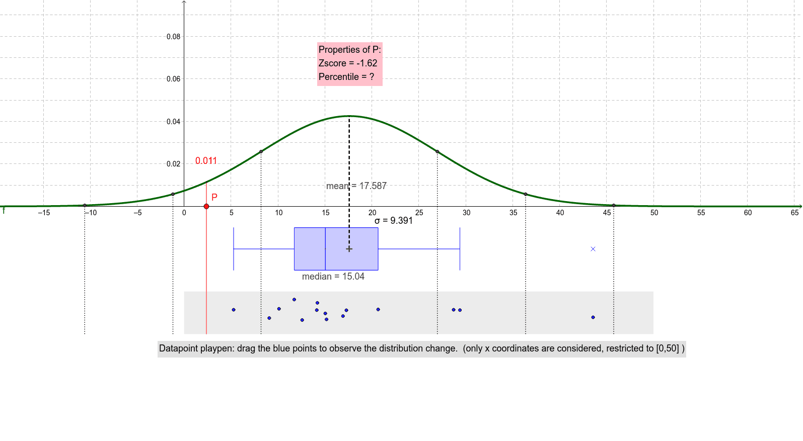
This example demonstrates how moving discrete data points affects the distribution shape. Core math concepts include distribution, mean, standard deviation, and box plot. Construction involves commands like Polygon, PointIn, SD, Mean, Normal, BoxPlot, Segment, Intersect, Point, OrthogonalLine, Mirror, Integral, and objects S, R, Q, P_1, etc. Suitable for high school and above to understand dynamic changes in data distribution, ideal for probability & statistics education.
GeoGebra Commands & Parameters
Polygon(P_1, Q, R, S) → poly1, p, q, r, sPointIn(poly1) → BPointIn(poly1) → CPointIn(poly1) → DPointIn(poly1) → EPointIn(poly1) → FPointIn(poly1) → GPointIn(poly1) → HPointIn(poly1) → IPointIn(poly1) → JPointIn(poly1) → KPointIn(poly1) → LPointIn(poly1) → MPointIn(poly1) → NPointIn(poly1) → OPointIn(poly1) → ASD(X) → sdMean(X) → meanNormal(mean, sd, x) → fBoxPlot(-0.02, 0.01, X, true) → medianSegment(T, U) → aIntersect(a, xAxis) → VPoint(xAxis) → POrthogonalLine(P, xAxis) → bPoint(Circle[V, abs(sd)]) → SD_1Segment(V, SD_1) → cPoint(Circle[V, abs((2 * sd))]) → SD_2Segment(V, SD_2) → dPoint(Circle[V, abs((3 * sd))]) → SD_3Segment(V, SD_3) → eOrthogonalLine(SD_1, xAxis) → gOrthogonalLine(SD_2, xAxis) → hOrthogonalLine(SD_3, xAxis) → iMirror(SD_1, a) → SD_n1Mirror(SD_2, a) → SD_n2Mirror(SD_3, a) → SD_n3OrthogonalLine(SD_n3, xAxis) → jOrthogonalLine(SD_n2, xAxis) → kOrthogonalLine(SD_n1, xAxis) → lIntegral(f, -Infinity, x(P)) → mIntersect(f, l, (8.196150479331507, 0.025765600325250028)) → ZIntersect(f, k, (-1.1950812973259275, 0.005749082526893479)) → A_1Intersect(f, j, (-10.58631307398337, 4.7191343130873153E-4)) → B_1Intersect(f, g, (26.97861403264639, 0.025765600325250028)) → C_1Intersect(f, h, (36.369845809303825, 0.005749082526893479)) → D_1Intersect(f, i, (45.76107758596127, 4.7191343130873153E-4)) → E_1Intersect(j, t) → F_1Intersect(k, t) → G_1Intersect(l, t) → H_1Intersect(g, t) → I_1Intersect(h, t) → J_1Intersect(i, t) → K_1Intersect(b, t) → L_1Intersect(f, b, (2.3743156048055805, 0.011438284314040505)) → M_1Segment(F_1, B_1) → a_1Segment(G_1, A_1) → b_1Segment(L_1, M_1) → c_1Segment(H_1, Z) → d_1Segment(I_1, C_1) → e_1Segment(J_1, D_1) → f_1Segment(K_1, E_1) → g_1
AI Drawing Prompt Reference
Draw a polygon with randomly generated points inside to show how moving these points affects data distribution. Calculate the mean and standard deviation of the points, plot a normal distribution curve to represent the data distribution, and create a box plot. Mark the mean and standard deviation on the coordinate axis, and draw corresponding standard deviation lines. Finally, complete the graphic display through integration and reflection operations.
The prompt above was compiled from the original drawing commands and is for reference only.