
Display and Compare Two Proper Fractions
Loading the math board and drawing, please wait…
In collections
fifth grade fractions
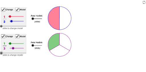
This example demonstrates multiple representations of two different proper fractions, including linear, number line, and set models. Students can better understand the concept of proper fractions and their geometric meanings through these different representations. The construction uses commands such as Point, Min, If, Vector, Rotate, CircleSector, Segment, Polygon, Sequence, Circle, and FractionText in GeoGebra. Suitable for students from upper elementary to middle school, it helps develop students' geometric intuition and mathematical thinking.
GeoGebra Commands & Parameters
Point(Circle[R_1, 0.12]) → C_2Min(9 / denom1, 1) → a9Min(4 / denom1, 1) → a4Min(5 / denom1, 1) → a5Min(8 / denom1, 1) → a8Min(7 / denom1, 1) → a7Min(6 / denom1, 1) → a6Min(1 / denom1, 1) → a1Min(2 / denom1, 1) → a2If(denom1 < 10, " " + denom1, "" + denom1) → formatdMin(3 / denom1, 1) → a3Min(10 / denom1, 1) → a10Point(Circle[M, 1]) → QPoint(Circle[N, 1]) → RPoint(Circle[L_1, 0.02]) → U_1Point(Circle[U_1, 0.5]) → V_1If(impr > 1, 1, 0) → Rect_{show}Vector(NL_c, NL_l) → uVector(NL_c, NL_r) → vIf(num1 / denom1 > 1, 1, 0) → Set_{show}Rotate(C_2, angle, R_1) → D_2CircleSector(R_1, C_2, D_2) → circle1_{sector}Rotate(C_2, (360 / denom1)°, R_1) → B_2Segment(K_2, L_2) → a_2Vector((0, 0.25), (0.1, 0.25)) → image_{vector}Polygon((0, 0.38), ((0.5 * num1 / denom1), 0.38), ((0.5 * num1 / denom1), 0.58), (0, 0.58)) → frac1area3_{shaded}, j_1, k_1, l_1, m_1Segment((1, 0.43), (1, 0.47)) → i_2Sequence(Segment[((1 / frac1linediv * i), 0.43), ((1 / frac1linediv * i), 0.47)], i, 1, frac1linediv) → frac1numLineHashSegment((0, 0.42), (0, 0.48)) → t_1Segment((1, 0.42), (1, 0.48)) → aPolygon((0, 0.38), (num1 / 10, 0.38), (num1 / 10, 0.58), (0, 0.58)) → frac1area2_{shaded}, b, c, d, eSequence(Segment[(i / denom1, 0.42), (i / denom1, 0.48)], i, 1, denom1 - 1) → frac1linearModelDivisionsPolygon((0, 0.42), (num1 / denom1, 0.42), (num1 / denom1, 0.48), (0, 0.48)) → frac1linear_{shaded}, f, g, h, iSequence(Translate[Circle[(0.05, 0.48), 0.045], Vector[(0, 0), ((0.1 * i), 0)]], i, 0, denom1 - 1) → frac1OpenCirclesSequence(Translate[Circle[(0.05, 0.48), 0.04], Vector[(0, 0), ((0.1 * i), 0)]], i, 0, num1 - 1) → frac1setClosedSequence(Segment[Rotate[(0.1504, 0.2), (360 / denom1)°, (0.1504, 0.2)], Rotate[(0.1504, 0.31), ((360 * i) * ° / denom1), (0.1504, 0.2)]], i, 0, denom2 - 1) → Circle2_{model-divisions}Circle((0.15, 0.2), 0.12) → Circle2_{outline}Sequence(Segment[Rotate[(0.15, 0.2), ((360 / denom1 * i))°, (0.15, 0.2)], Rotate[(0.15, 0.32), ((360 * i / denom2))°, (0.15, 0.2)]], i, 0, denom2) → circle2_{div}Circle((0.15, 0.475), 0.12) → Circle1_{outline}Sequence(Segment[Rotate[(0.15, 0.475), ((360 / denom1 * i))°, (0.15, 0.475)], Rotate[(0.15, 0.595), ((360 * i / denom1))°, (0.15, 0.475)]], i, 0, denom1) → circle1_{div}CircleSector((0.15, 0.2), (0.15, 0.32), Rotate[(0.15, 0.32), ((360 * num2 / denom2))°, (0.15, 0.2)]) → pPolygon((0, 0.38), (denom1 / 10, 0.38), (denom1 / 10, 0.58), (0, 0.58)) → frac1area2_{outline}, r, s, t, a_1Sequence(Segment[(i / 10, 0.38), (i / 10, 0.58)], i, 1, denom1 - 1) → frac1area_{div}Polygon((0, 0.1), (denom2 / 10, 0.1), (denom2 / 10, 0.3), (0, 0.3)) → frac2area2_{outline}, j, l, n, qSequence(Segment[(i / 10, 0.1), (i / 10, 0.3)], i, 1, denom2 - 1) → frac2area_{div}Polygon((0, 0.1), (num2 / 10, 0.1), (num2 / 10, 0.3), (0, 0.3)) → frac2area2_{shaded}, b_1, c_1, d_1, e_1Polygon((0, 0.38), (0.5, 0.38), (0.5, 0.58), (0, 0.58)) → frac1area3_{outline}, f_1, g_1, h_1, i_1Polygon((0, 0.1), (0.5, 0.1), (0.5, 0.3), (0, 0.3)) → frac2area3_{outline}, n_1, p_1, q_1, r_1Sequence(Segment[((0.5 / denom1 * i), 0.38), ((0.5 / denom1 * i), 0.58)], i, 1, denom1 - 1) → frac1area3_{div}Sequence(Segment[((0.5 / denom2 * i), 0.1), ((0.5 / denom2 * i), 0.3)], i, 1, denom2 - 1) → frac2area3_{div}Polygon((0, 0.1), ((0.5 * num2 / denom2), 0.1), ((0.5 * num2 / denom2), 0.3), (0, 0.3)) → frac2area3_{shaded}, s_1, b_2, c_2, d_2Sequence(Translate[Circle[(0.05, 0.2), 0.04], Vector[(0, 0), ((0.1 * i), 0)]], i, 0, num2 - 1) → frac2setClosedSequence(Translate[Circle[(0.05, 0.2), 0.045], Vector[(0, 0), ((0.1 * i), 0)]], i, 0, denom2 - 1) → frac2setOpenVector(NL_c + (0, -0.27), NL_l + (0, -0.27)) → u_1Vector(NL_c + (0, -0.27), NL_r + (0, -0.27)) → v_1Segment((0, 0.43), (0, 0.47)) → f_2Segment((0, 0.16), (0, 0.2)) → e_2Segment((1, 0.16), (1, 0.2)) → g_2Sequence(Segment[((1 / frac2linediv * i), 0.16), ((1 / frac2linediv * i), 0.2)], i, 1, frac2linediv) → frac2numLineHashVector(Frac2NumLnPt + (0, 0.05), Frac2NumLnPt) → frac2NumLnPtVectorVector(Frac1NumLnPt + (0, 0.05), Frac1NumLnPt) → frac1NumLnPtVectorFractionText(1 / frac2linediv) → model2NumLnIntervalValueFractionText(1 / frac1linediv) → model1NumLnIntervalValueSegment(K_2 + (0, -0.27), L_2 + (0, -0.27)) → h_2Sequence(Segment[(i / denom2, 0.15), (i / denom2, 0.21)], i, 1, denom2 - 1) → frac2linearModelDivisionsSegment((1, 0.15), (1, 0.21)) → j_2Segment((0, 0.15), (0, 0.21)) → k_2Polygon((0, 0.15), (num2 / denom2, 0.15), (num2 / denom2, 0.21), (0, 0.21)) → frac2linear_{shaded}, l_2, m_2, n_2, p_2Sequence(Polygon[(-0.455, 0.117 + k), (-0.195, 0.117 + k), (-0.195, 0.31 + k), (-0.455, 0.31 + k)], k, 0, 0.276, 0.276) → grayBoxesSequence(Segment[(-0.435, 0.189 + k), (-0.397, 0.189 + k)], k, 0, 0.276, 0.276) → fracVinculum
AI Drawing Prompt Reference
Draw multiple representations of two proper fractions, including set models, linear models, and geometric models. Start by drawing two circles to represent the set models of the fractions. Then, draw two number lines to represent the linear models of the fractions. Next, draw two sectors to represent the geometric models of the fractions. Finally, use rectangles and polygons to shade the areas corresponding to each fraction.
The prompt above was compiled from the original drawing commands and is for reference only.