
Directional Derivatives Demo by Mike Hopper
Loading the math board and drawing, please wait…
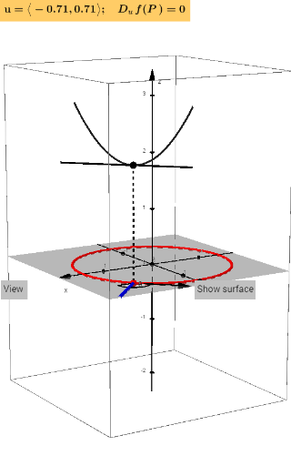
This example demonstrates the geometric interpretation of directional derivatives, visualizing the rate of change of a function at a point along any direction. Key math concepts include derivatives, vectors, gradients, and function graphs. Construction highlights the use of GeoGebra commands and objects like Circle, Point, Vector, Function, Derivative, grad to build the function graph, gradient vectors, and directional derivative lines. Suitable for university calculus courses or math enthusiasts to gain an intuitive understanding of directional derivatives.
GeoGebra Commands & Parameters
Circle(P, 1) → tPoint(t) → BDerivative(f(x, y), x) → fxDerivative(f(x, y), y) → fyVector(P, P + (fx(x(P), y(P)), fy(x(P), y(P)))) → gradImplicitCurve(f(x, y) - f(x(P), y(P))) → cImplicitCurve(f(x, y)) → dImplicitCurve(f(x, y) - 1) → gImplicitCurve(f(x, y) - 2) → hImplicitCurve(f(x, y) - 3) → iImplicitCurve(f(x, y) - 4) → jImplicitCurve(f(x, y) - 5) → kImplicitCurve(f(x, y) + 1) → lImplicitCurve(f(x, y) + 2) → mImplicitCurve(f(x, y) + 3) → nImplicitCurve(f(x, y) + 4) → oImplicitCurve(f(x, y) + 5) → pPlane(P, P', P + (fx(x(P), y(P)), fy(x(P), y(P)))) → rCurveCartesian(x(P) + (fx(x(P), y(P)) * w), y(P) + (fy(x(P), y(P)) * w), w, -100, 100) → qCurveCartesian(x(P') + (fx(x(P), y(P')) * Q), y(P') + (fy(x(P), y(P)) * Q), z(P') + ((fx(x(P), y(P))^(2) + fy(x(P), y(P))^(2)) * Q), Q, -100, 100) → eTextfield(f) → InputBox1Textfield(Px) → InputBox2Textfield(Py) → InputBox3Length(grad) → normgradSegment(P'', P') → sFunction(f(x(P'), y(P')) + (fx(x(P'), y(P')) * (x - x(P'))) + (fy(x(P'), y(P')) * (y - y(P'))), x(P) - 1, x(P) + 1, y(P) - 1, y(P) + 1) → bRotate(B, θ, P) → AVector(P, A) → uOrthogonalLine(P, u, xOyPlane) → f_1OrthogonalPlane(P'', f_1) → vIntersectPath(v, f) → wIntersectPath(v, b) → a_1Angle(B, P, A) → βTextfield(θ) → InputBox4Point(zAxis) → CIntersect(zAxis, xAxis) → DVector(C, D) → u_1Point(yAxis) → EVector(E, D) → v_1Point(xAxis) → FVector(F, D) → w_1Element(list1, faces) → Selectedvector
AI Drawing Prompt Reference
Draw a function graph and show its gradient vector and directional derivatives at a point. Start by plotting the origin and drawing a circle around it, connecting points on the circle to the origin to form vectors. Then, based on the partial derivatives at the point, draw the gradient vector and implicit curves for the function's contour lines. Add multiple parallel curves to represent different heights. Finally, from the gradient vector, draw directional derivative lines along arbitrary directions to show the rate of change of the function in those directions.
The prompt above was compiled from the original drawing commands and is for reference only.