
Dilation Transformation Demo by Emily Brown
Loading the math board and drawing, please wait…
In collections
Dilations
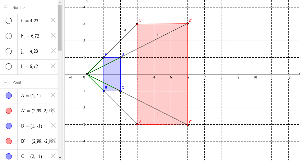
This example demonstrates how to perform similarity transformations (scaling) in geometry by observing the changes in a figure after transformation to understand the properties of similarity transformations. The core math concepts involved include scale factor, central symmetry, and the angle-preserving property of figures. Construction highlights: Polygon, Intersect, Segment, Point commands are used; suitable for high school geometry teaching to help students visually grasp similarity transformations.
GeoGebra Commands & Parameters
Polygon(A, B, C, D) → poly1, a, b, c, dIntersect(xAxis, yAxis) → ESegment(E, A) → ePoint(Circle[E, 4.23]) → A'Segment(E, A') → fSegment(E, D) → gPoint(Circle[E, 6.720000000000001]) → D'Segment(E, D') → hSegment(E, B) → iPoint(Circle[E, 4.2299999999999995]) → B'Segment(E, B') → jSegment(E, C) → kPoint(Circle[E, 6.72]) → C'Segment(E, C') → lPolygon(A', B', C', D') → poly2, a', b', c', d'
AI Drawing Prompt Reference
Draw a quadrilateral with its four vertices connected by line segments to the origin point where the axes intersect. On each segment, place a new point at a scaled distance from the origin (some closer, some farther), then connect these four new points to form a second quadrilateral. Both quadrilaterals share the same center, with corresponding vertices lying on the same rays, illustrating a dilation transformation.
The prompt above was compiled from the original drawing commands and is for reference only.