
Digital Clocks: Standard Time and Number Theory Madness
Loading the math board and drawing, please wait…
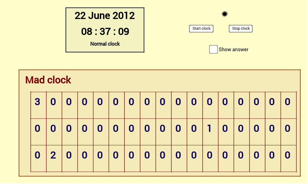
This GeoGebra example demonstrates two distinct styles of digital clocks: a standard digital clock utilizing the straightforward `GetTime[]` command, and a "mad" clock that playfully integrates number theory into timekeeping. The core mathematical concepts involved include arithmetic, prime factorization, prime numbers, and logical conditional structures representing hours, minutes, and seconds. To construct this, the creator used a combination of GeoGebra commands such as `Element`, `If`, `Factors`, `Zip`, `Polygon`, `Sequence`, and `Segment`. Key objects include `hrs`, `min`, `sec`, `primes`, and various factorization variables like `myFactors`, `secFac`, and `hrsOut`, which dynamically compute the visual segments of the digits. Interactive buttons `button1` and `button2` allow users to toggle between the standard and the number theory-based visualizations. This resource is highly suitable for high school and college-level students, logic puzzle enthusiasts, and anyone interested in the creative intersection of number theory and graphical visualization.
GeoGebra Commands & Parameters
Element(tmp, 2) → secElement(tmp, 4) → hrsElement(tmp, 3) → minElement(tmp, 5) → dayElement(tmp, 6) → mntElement(tmp, 8) → mnttIf(hrs < 10, "0" + hrs, "" + hrs) → hrstIf(min < 10, "0" + min, "" + min) → mintIf(sec < 10, "0" + sec, "" + sec) → sectFactors(If[z < 3, 2, z]) → myFactorsZip(Element[a, 2], a, myFactors[sec]) → secPowZip(Element[a, 1], a, myFactors[sec]) → secFacZip(If[(IndexOf[p, secFac] > 0) ∧ (sec > 1), Element[secPow, IndexOf[p, secFac]], 0], p, primes) → secOutZip(Element[a, 1], a, myFactors[min]) → minFacZip(Element[a, 2], a, myFactors[min]) → minPowZip(Element[a, 2], a, myFactors[hrs]) → hrsPowZip(Element[a, 1], a, myFactors[hrs]) → hrsFacZip(If[(IndexOf[p, hrsFac] > 0) ∧ (hrs > 1), Element[hrsPow, IndexOf[p, hrsFac]], 0], p, primes) → hrsOutZip(If[(IndexOf[p, minFac] > 0) ∧ (min > 1), Element[minPow, IndexOf[p, minFac]], 0], p, primes) → minOutPolygon((0, -1), (0, 5), (18, 5), (18, -1)) → poly2, e, f, g, hPolygon((3, 6), (3, 8.5), (8, 8.5), (8, 6)) → poly1, a, b, c, dFactors(59) → matrix1Sequence(Text[Element[hrsOut, k], (k, 3)], k, 1, 17) → hrsShowSequence(Text[Element[minOut, k], (k, 1.5)], k, 1, 17) → minShowSequence(Text[Element[secOut, k], (k, 0)], k, 1, 17) → secShowSequence(Text[Element[primes, k] + "^" + (Element[hrsOut, k]) + "\cdot", (k, 2.75), true, true], k, 1, 17) → hrsFullSequence(Text[Element[primes, k] + "^" + (Element[minOut, k]) + "\cdot", (k, 1.25), true, true], k, 1, 17) → minFullSequence(Text[Element[primes, k] + "^" + (Element[secOut, k]) + "\cdot", (k, -0.25), true, true], k, 1, 17) → secFullSegment((0.75, -0.75), (17.75, -0.75)) → r1Segment((0.75, 0.75), (17.75, 0.75)) → r2Segment((0.75, 2.25), (17.75, 2.25)) → r3Segment((0.75, 3.75), (17.75, 3.75)) → r4Sequence(Segment[(j, -0.75), (j, 3.75)], j, 0.75, 17.75) → r
AI Drawing Prompt Reference
Draw a dual-mode digital clock showing the current time both as ordinary digits and as a prime-factorization table. The scene contains two rectangular panels: the upper panel displays hours, minutes, and seconds in standard 24-hour format with leading zeros; the lower panel lists the first seventeen primes horizontally, and for each prime shows the exponent appearing in the factorization of the hour, minute, and second values (zero exponents omitted). Three rows of text below the primes present the full factor products for hours, minutes, and seconds. A series of evenly spaced vertical segments forms a grid aligning the prime columns. Two toggle buttons let the user switch between the plain digital view and the number-theory view.
The prompt above was compiled from the original drawing commands and is for reference only.