
Different Prices: Function Graphs and Expected Value Comparison
Loading the math board and drawing, please wait…
In collections
LINEAR FUNCTIONS
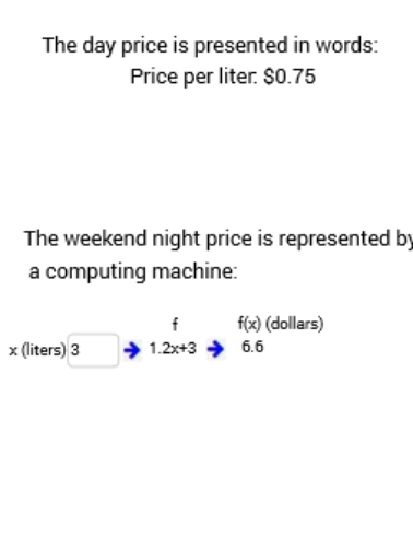
This GeoGebra example dynamically illustrates how different price settings affect function graphs and expected values. Core mathematical concepts include function graphing, polynomial functions, exponential functions, and expected value calculation. The construction uses text fields and input boxes for price parameters, points, lines, orthogonal lines, segments, polygons for geometric aids, and table text for data display. Suitable for high school or pre-university students learning function modeling and expected value in probability and statistics, as well as for classroom demonstrations of how price changes impact economic models.
GeoGebra Commands & Parameters
Textfield(a) → InputBox1Point(xAxis) → GPoint(xAxis) → HLine(G, H) → fPoint(yAxis) → IPoint(yAxis) → JLine(I, J) → gOrthogonalLine(K, g) → hOrthogonalLine(K, h) → iSegment(L, K) → jPolygon((0, 0), (0, 10), (8, 10), (8, 0)) → poly1, k, l, m, nTableText({{A1, B1}, {A2, B2}, {A3, B3}, {A4, B4}, {A5, B5}}, "|_") → text9Textfield(c) → InputBox2
AI Drawing Prompt Reference
Draw a coordinate plane with a rectangular region as background. Place two movable points on the x-axis and connect them to form a line; place two movable points on the y-axis and connect them to form another line. From a point outside the rectangle, draw a perpendicular to the first line, then a perpendicular to that perpendicular, creating two orthogonal auxiliary lines. Connect a point inside the rectangle to an external point with a segment. Include two input boxes for adjusting price parameters, and display a table showing function values and expected values for different prices. Overall, illustrate how price changes affect function graphs and expected outcomes.
The prompt above was compiled from the original drawing commands and is for reference only.