
Dependence of Average Distance on Truncation Parameter in Truncated Square Antip
Loading the math board and drawing, please wait…
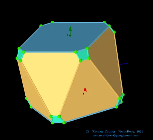
This example demonstrates how the average distance between vertices of a truncated square antiprism depends on the truncation parameter. By adjusting the truncation parameter, the extreme distribution of vertices can be observed. Commands used include Join, Unique, Length, Text, Sum, Sphere, Ray, Zip, UnicodeToLetter, TableText, etc. Suitable for high school mathematics education, particularly in coordinate geometry and solid geometry.
GeoGebra Commands & Parameters
Join(Zip[lP0(x(a)) + ((lP0(y(a)) - lP0(x(a))) * {t, 1 - t}), a, segN]) → lVVUnique(lVV) → lP'Length(lP') → nLength(lVV(1)) → R2Text("" + p3) → txt_pSum(Flatten[Sequence[Append[Sequence[Element[txt_p, i], i, m1(k), m2(k)], " "], k, 1, 5]]) → txtUm1Sphere(O, R1) → sp1Sphere(O, R2) → sp2Ray(B, AA) → hText(text12, C, false, true) → text8Zip(Polygon[a], a, v_poly08) → poly08Zip(Segment[lP0(x(a)), lP0(y(a))], a, segN1) → seg1Zip(Segment[lP0(x(a)), lP0(y(a))], a, segN2) → seg2Zip(Polygon[a], a, v_poly04) → poly04Zip(Polygon[a], a, v_poly06) → poly06UnicodeToLetter(34) → u34Zip(Segment[lVV(x(a)), lVV(y(a))], a, segNΔ4) → segΔ4Zip(Segment[lVV(x(a)), lVV(y(a))], a, segNΔ8) → segΔ8Zip(Segment[lVV(x(a)), lVV(y(a))], a, segNΔ6) → segΔ6TableText(Append["\;\;\; \fgcolor{#08E8DE}{4-gons}", segΔ4], Append["\;\;\; \fgcolor{#B5A642}{6-gons}", segΔ4], Append["\;\;\; \fgcolor{#007FFF}{8-gons}", segΔ8], "v") → text3a