
Demonstration of Solutions to sin x = a
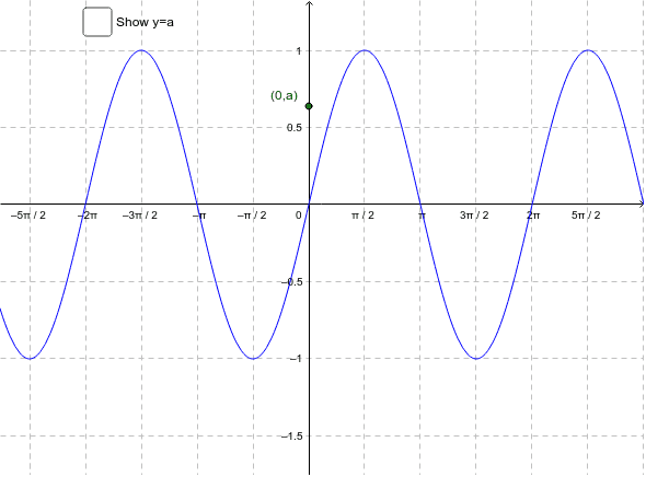
Loading the math board and drawing, please wait…
This example demonstrates the solutions to the equation sin x = a as the value of a changes, illustrating key trigonometric concepts and coordinate geometry. It constructs key points and trajectories using GeoGebra commands like Point, OrthogonalLine, Corner, Intersect, and Sequence. Suitable for high school trigonometry instruction.
GeoGebra Commands & Parameters
Point(yAxis) → AOrthogonalLine(A, yAxis) → aCorner(1) → corner1Corner(2) → corner2Corner(3) → corner3Corner(4) → corner4Intersect(f, a, (789968.4884233484, 0.6382978723179175)) → solSequence(Segment[(((2 * n) * π) + x(sol), y(sol)), (((2 * n) * π) + x(sol), 0)], n, round((x(Corner[1]) - x(sol)) / ((2 * π))), round((x(Corner[2]) - x(sol)) / ((2 * π))), 1) → solutionsSequence(Segment[(((2 * n) * π) + π - x(sol), y(sol)), (((2 * n) * π) + π - x(sol), 0)], n, round((x(Corner[1]) - π + x(sol)) / ((2 * π))), round((x(Corner[2]) - π + x(sol)) / ((2 * π))), 1) → solutions2
AI Drawing Prompt Reference
Draw a sine function graph and demonstrate how the solutions to the equation sin x = a change as the parameter a varies. Start by plotting the y-axis and marking a point on it, then draw a perpendicular line from this point to determine the value of a. Next, find the intersection point on the sine function graph corresponding to the parameter a, and use this point to draw two trajectory segments along the periodic sine function, representing the solutions. Finally, connect these solutions with line segments to show their distribution pattern.
The prompt above was compiled from the original drawing commands and is for reference only.