
Demonstration of Slopes in Function Composition
Loading the math board and drawing, please wait…
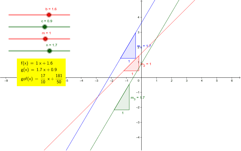
This example illustrates the relationship between the slopes of composite linear functions. Key math concepts include function composition, linear function slopes, and the product rule for slopes. GeoGebra commands used are Expand, TableText, Point, Line, and Slope, along with objects like m, n, b, c, f, g, h, gof, text1, A, B, a, C, D, d, E, F, e, m_1, m_2, m_3. It is suitable for high school mathematics instruction on understanding function composition and slope calculations.
GeoGebra Commands & Parameters
Expand(h) → gofTableText({{LaTeX[f, true, true]}, {LaTeX[g, true, true]}, {LaTeX[gof, true, true]}}) → text1Point(gof) → APoint(gof) → BLine(A, B) → aPoint(f) → CPoint(f) → DLine(C, D) → dPoint(g) → EPoint(g) → FLine(E, F) → eSlope(a) → m_1Slope(d) → m_2Slope(e) → m_3
AI Drawing Prompt Reference
Draw two linear functions f and g, and their composition gof. First, plot f and g, then plot gof. Calculate and display the slopes m1, m2, and m3 of f, g, and gof respectively.
The prompt above was compiled from the original drawing commands and is for reference only.