
Cylinder Volume Calculation & Visualization
Loading the math board and drawing, please wait…
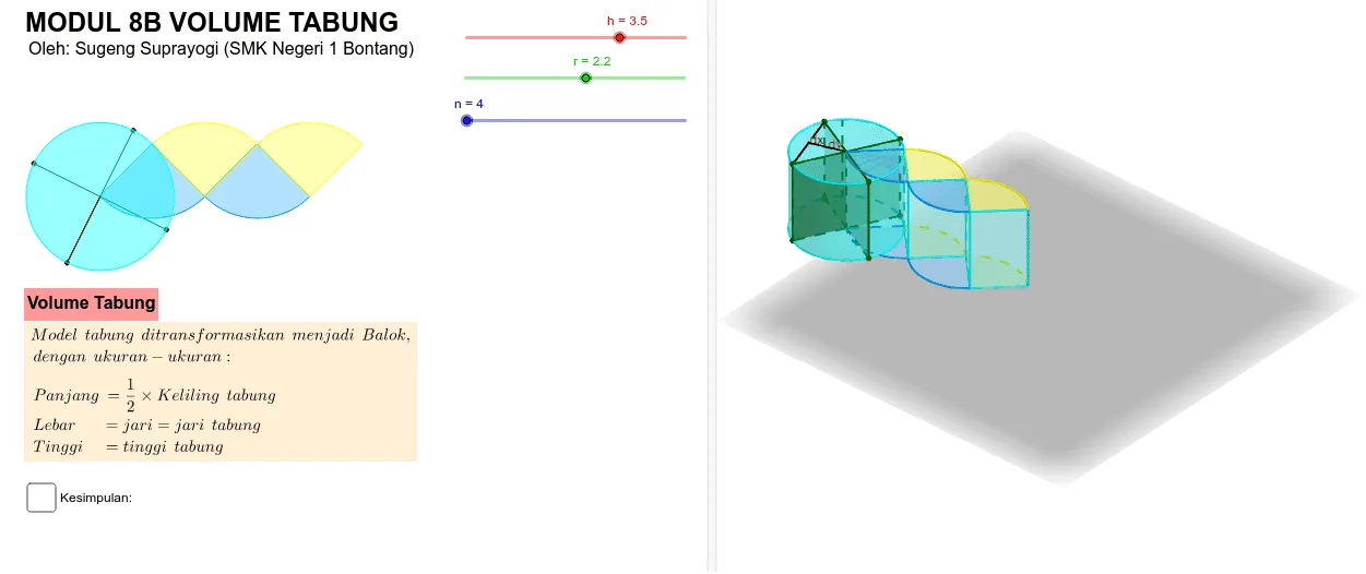
This example demonstrates the calculation and visualization of cylinder volume. It involves core math concepts like cylinder volume formula, geometric construction, and parametrization. GeoGebra commands used include Cylinder, Point, Ray, Line, Intersect, Segment, Polygon, Sequence, and OrthogonalLine. Suitable for high school students learning solid geometry and volume calculations, ideal for classroom demonstrations and interactive exploration.
GeoGebra Commands & Parameters
Cylinder(A, B, r) → a, c, d, bPoint(d) → CRay(B, C) → fLine(C, zAxis) → gIntersect(g, c) → D,Segment(B, C) → iSegment(A, D) → j_1Segment(C, D) → kPolygon(A, B, C, D) → q1, a_1, b_1, c_1, d_1Line(A, B) → jSequence(Rotate[C, ((i * 360) * ° / n), B], i, 0, n) → L_1Sequence(Rotate[D, ((i * 360) * ° / n), A], i, 0, n) → L_2Sequence(Segment[Rotate[C, ((i * 360) * ° / n), B], Rotate[D, ((i * 360) * ° / n), A]], i, 0, n) → L_3Sequence(Segment[Rotate[B, ((i * 360) * ° / n), B], Rotate[C, ((i * 360) * ° / n), B]], i, 0, n) → L_4Sequence(Segment[Rotate[A, ((i * 360) * ° / n), B], Rotate[D, ((i * 360) * ° / n), B]], i, 0, n) → L_5Sequence(Rotate[q1, ((i * 360) * ° / n), j], i, 0, n) → L_6Point(d) → GSegment(C, G) → lOrthogonalLine(B, l, space) → mIntersect(m, l) → HSegment(B, H) → pSegment(C, G) → dxSegment(B, H) → dySequence(CircleSector[((j * dx) + dx / 2, dy), ((j * dx) + 0, 0), ((j * dx) + dx, 0)], j, 0, n / 2 - 1) → L_7Sequence(CircleSector[((j * dx), 0), ((j * dx) + dx / 2, dy), ((j * dx) + ((-dx)) / 2, dy)], j, 1, n / 2) → L_8Sequence(CircleSector[((j * dx) + dx / 2, dy, h), ((j * dx) + 0, 0, h), ((j * dx) + dx, 0, h), xOyPlane], j, 0, n / 2 - 1) → L_9Sequence(CircleSector[((j * dx), 0, h), ((j * dx) + dx / 2, dy, h), ((j * dx) + ((-dx)) / 2, dy, h), xOyPlane], j, 1, n / 2) → L_{10}Sequence(Segment[((i * dx), 0, 0), ((i * dx), 0, h)], i, 0, n / 2) → L_{11}Sequence(Segment[((i * dx) - dx / 2, dy, 0), ((i * dx) - dx / 2, dy, h)], i, 0, n / 2 + 1) → L_{12}Sequence(Polygon[((((2 * i) - 1) * dx / 2), dy, 0), ((((2 * i) - 1) * dx / 2), dy, h), ((i * dx), 0, h), ((i * dx), 0, 0)], i, 1, n / 2) → L_{13}Sequence(Polygon[((((2 * i) + 1) * dx / 2), dy, h), ((((2 * i) + 1) * dx / 2), dy, 0), ((i * dx), 0, 0), ((i * dx), 0, h)], i, 1, n / 2) → L_{14}
AI Drawing Prompt Reference
Draw a cylinder to visualize its volume calculation. Start by creating the base and side of the cylinder. Then, draw a ray from the center of the base to the side, find the intersection point between the ray and the cylinder's side. Connect the base center to this intersection point to form a quadrilateral. Finally, rotate this quadrilateral around the cylinder's axis to generate multiple similar quadrilaterals, representing the side's unfolding, and use sectors to show small sections of the side for a clear volume calculation demonstration.
The prompt above was compiled from the original drawing commands and is for reference only.