
Cumulative Frequency Distributions
Loading the math board and drawing, please wait…
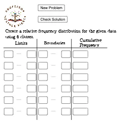
This example demonstrates how to create a cumulative frequency distribution using GeoGebra, involving core concepts like frequency distribution, statistics, scatter plots, and linear equations. Key GeoGebra commands and objects used include Random, Min, Max, Textfield, Segment, CountIf, and data points A1-A11, B1-B11, C1-C11 for constructing the plot and cumulative frequency line. Suitable for high school statistics education or introductory data analysis learning.
GeoGebra Commands & Parameters
Random(50, 99) → A1Random(50, 99) → B1Random(50, 99) → C1Random(50, 99) → C2Random(50, 99) → B2Random(50, 99) → A2Random(50, 99) → A3Random(50, 99) → B3Random(50, 99) → C3Random(50, 99) → C4Random(50, 99) → B4Random(50, 99) → A4Random(50, 99) → A5Random(50, 99) → B5Random(50, 99) → C5Random(50, 99) → C6Random(50, 99) → B6Random(50, 99) → A6Random(50, 99) → A7Random(50, 99) → B7Random(50, 99) → C7Random(50, 99) → C8Random(50, 99) → B8Random(50, 99) → A8Random(50, 99) → A9Random(50, 99) → B9Random(50, 99) → C9Random(50, 99) → C10Random(50, 99) → B10Random(50, 99) → A10Random(50, 99) → A11Random(50, 99) → B11Random(50, 99) → C11Random(50, 99) → C12Random(50, 99) → B12Random(50, 99) → A12Random(50, 99) → A13Random(50, 99) → B13Random(50, 99) → C13Random(50, 99) → C14Random(50, 99) → B14Random(50, 99) → A14Random(50, 99) → A15Random(50, 99) → B15Random(50, 99) → C15Min(Data) → minMax(Data) → maxTextfield(lower1) → InputBox1Textfield(lower2) → InputBox2Textfield(lower3) → InputBox3Textfield(lower4) → InputBox4Textfield(lower5) → InputBox5Textfield(lower6) → InputBox6Textfield(upper1) → InputBox7Textfield(upper2) → InputBox8Textfield(upper3) → InputBox9Textfield(upper4) → InputBox10Textfield(upper5) → InputBox11Textfield(upper6) → InputBox12Segment(A, B) → fSegment(C, D) → gTextfield(lboundary1) → InputBox13Textfield(lboundary2) → InputBox14Textfield(lboundary3) → InputBox15Textfield(lboundary4) → InputBox16Textfield(lboundary5) → InputBox17Textfield(lboundary6) → InputBox18Textfield(uboundary1) → InputBox19Textfield(uboundary2) → InputBox20Textfield(uboundary3) → InputBox21Segment(E, F) → hTextfield(frequency1) → InputBox25Textfield(frequency2) → InputBox26Textfield(frequency3) → InputBox27Textfield(frequency4) → InputBox28Textfield(frequency5) → InputBox29Textfield(frequency6) → InputBox30Textfield(uboundary4) → InputBox22Textfield(uboundary5) → InputBox23Textfield(uboundary6) → InputBox24CountIf(l1 ≤ x ≤ u1, Data) → f1
AI Drawing Prompt Reference
Create a cumulative frequency distribution plot. Start by generating random data points on a coordinate plane, with both x and y coordinates ranging from 50 to 99, forming a scatter plot. Then compute the minimum and maximum of the data to set the axis limits. Next, draw a cumulative frequency line that starts at the minimum value and accumulates the count of data points in each interval up to the maximum, resulting in an ascending step-like or smooth curve. Finally, add a text input box near the graph to adjust the lower class boundary, allowing dynamic observation of the cumulative frequency distribution. The overall graph should include the scatter points, the cumulative frequency curve, and the interactive input box.
The prompt above was compiled from the original drawing commands and is for reference only.