Convergent Lens: Ray Path Demonstration

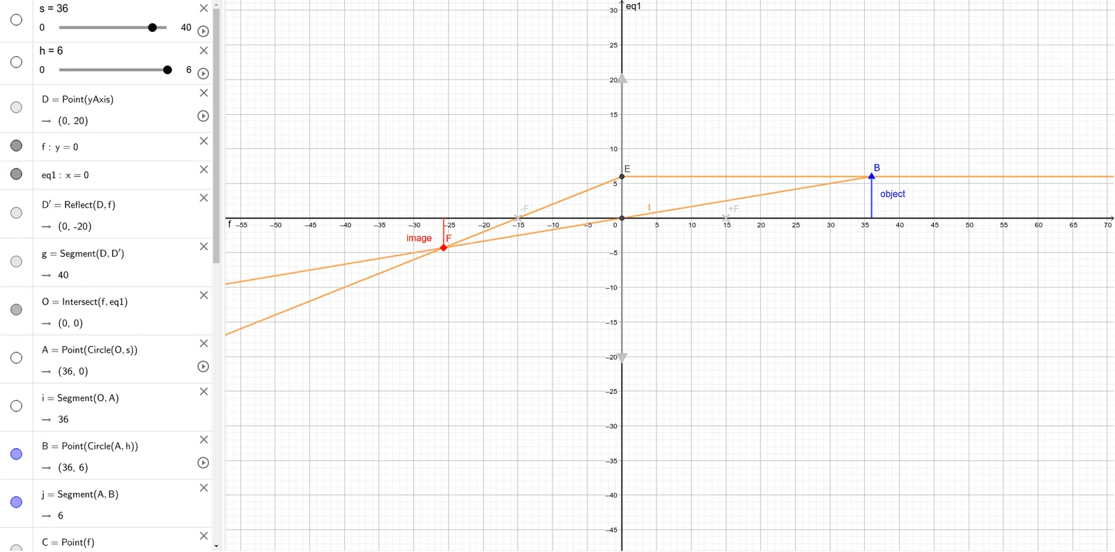
① This example visually demonstrates how a convergent (convex) lens focuses parallel rays and rays from a point source, showing the ray paths converging at the focal point. ② Core mathematical concepts include geometric optics, refraction law, focal point and focal length, optical axis and principal plane, and using symmetry and similar triangles to determine image positions. ③ Construction details: GeoGebra commands such as Point, Line, Ray for incident rays, OrthogonalLine for perpendicular auxiliary lines, Mirror for symmetry, Intersect for intersections, Segment for line segments, with objects s (lens), h (height), D (distance), f (focal length), eq1 (equation), D' (image point), g, O, A, i, B, j, C, F_2, k, E, l, m, F, n, G, p, q, r, t; dragging parameters dynamically updates the ray paths. ④ Suitable for high school physics optics, introductory university geometric optics, and as a GeoGebra demonstration for interactive learning of lens imaging rules.