
Confidence Intervals Visualization
Loading the math board and drawing, please wait…
In collections
Confidence Intervals
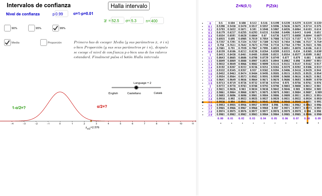
This example demonstrates how to create and visualize confidence intervals using GeoGebra, covering core math concepts like confidence intervals, polygons, cylinders, linear equations, Pythagorean theorem, and statistical characteristics. It utilizes commands such as Normal, Textfield, Sequence, TableText, Append, Integral, Element, and Segment for construction. Suitable for high school students and educators needing to understand statistical inference concepts.
GeoGebra Commands & Parameters
Normal(0, 1, x) → fTextfield(nconf) → CasillaDeEntrada1Textfield(xbarra) → CasillaDeEntrada2Textfield(σ) → CasillaDeEntrada3Textfield(pr) → CasillaDeEntrada4Sequence(k, k, 0, 2.9, 0.1) → udecSequence(k, k, 0, 0.09, 0.01) → centSequence(Normal[0, 1, Element[udec, k] + Element[cent, 1]], k, 1, Length[udec]) → c1Sequence(Normal[0, 1, Element[udec, k] + Element[cent, 2]], k, 1, Length[udec]) → c2Sequence(Normal[0, 1, Element[udec, k] + Element[cent, 3]], k, 1, Length[udec]) → c3Sequence(Normal[0, 1, Element[udec, k] + Element[cent, 4]], k, 1, Length[udec]) → c4Sequence(Normal[0, 1, Element[udec, k] + Element[cent, 5]], k, 1, Length[udec]) → c5Sequence(Normal[0, 1, Element[udec, k] + Element[cent, 6]], k, 1, Length[udec]) → c6Sequence(Normal[0, 1, Element[udec, k] + Element[cent, 7]], k, 1, Length[udec]) → c7Sequence(Normal[0, 1, Element[udec, k] + Element[cent, 8]], k, 1, Length[udec]) → c8Sequence(Normal[0, 1, Element[udec, k] + Element[cent, 9]], k, 1, Length[udec]) → c9TableText({udec}, "vc_") → texto7Sequence(" " + (Text[Element[cent, k]]) + " ", k, 2, 10) → textocentAppend(" 0.00", textocent) → textocent2Sequence(Normal[0, 1, Element[udec, k] + Element[cent, 10]], k, 1, Length[udec]) → c10TableText({c1, c2, c3, c4, c5, c6, c7, c8, c9, c10}, "vc|_") → aulaTextfield(n) → CasillaDeEntrada5TableText({textocent2}, "hc") → texto8Sequence(A + (k / 29 * (B - A)), k, 0, 29) → verticalesSequence(C + (k / 9 * (D - C)), k, 0, 9) → horizontalesIntegral(f, -Infinity, z_{α/2}) → hIntegral(f, z_{α/2}, Infinity) → gElement(verticales, fila) → PfilaElement(horizontales, columna) → QcolumnaSegment(Pfila, PQ) → iSegment(Qcolumna, PQ) → j
AI Drawing Prompt Reference
Create a visualization of confidence intervals featuring a normal distribution curve and multiple intervals represented by colored lines, labeled with key values like mean and standard deviation. Start by drawing the normal curve, then construct the intervals based on input confidence levels, and finally add guide lines and text annotations.
The prompt above was compiled from the original drawing commands and is for reference only.