
Speed as the Derivative of Position
Loading the math board and drawing, please wait…
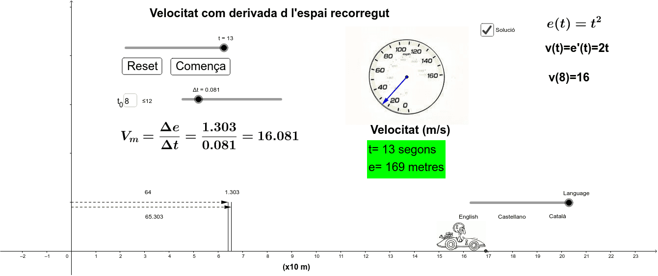
This example demonstrates the interpretation of the derivative as the speed of a vehicle. The core mathematical concept is the derivative. It uses Circle, Vector, Derivative, Rotate, Textfield, Segment, Midpoint, etc., GeoGebra commands/objects. Suitable for high school math education or learning the concept of derivatives.
GeoGebra Commands & Parameters
Circle(A, B) → cVector(A, B) → uDerivative(e) → vRotate(u, ((-3 * π / 2) * v(t) / 160)) → u'Textfield(t_0) → CajaDeEntrada1Segment((e_0, 0), (e_0, 2)) → aSegment((e_{t1}, 0), (e_{t1}, 2)) → bVector((0, 1.8), (e_{t1}, 1.8)) → wVector((0, 2), (e_0, 2)) → dMidpoint((e_0, 2), (e_{t1}, 2)) → C
AI Drawing Prompt Reference
Draw a coordinate plane illustrating the derivative of position as speed. Start with a circle centered at a point with another point on its circumference, and draw a vector from the center to that point. Add a curve representing position over time and its derivative curve. Rotate the vector by an angle proportional to the derivative value at a specific time to show velocity direction. Include a text input field to adjust the time parameter. Mark two time points on the horizontal axis, draw vertical segments of height 2 at each. From y=1.8, draw a horizontal vector to the second time point, and from y=2, draw a horizontal vector to the first time point, then mark the midpoint of these two vectors.
The prompt above was compiled from the original drawing commands and is for reference only.