Comparison of Means and SDs: Visualizing Data Variability

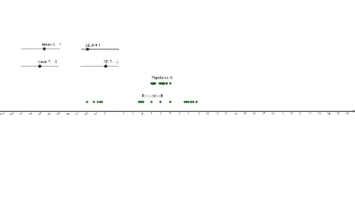
This GeoGebra example dynamically compares the means and standard deviations of two datasets (Group A and Group B), providing an intuitive visual understanding of central tendency and dispersion. It demonstrates how different data distributions can have similar means but different spreads, or vice versa. Core mathematical concepts include mean, standard deviation, data distribution, and the role of linear and polynomial functions in modeling trends. The construction uses GeoGebra commands such as Sequence to generate data series, Text for dynamic labels, and objects like PlotA, PlotB for data points, sA, sB for standard deviations, mA, mB for means, and PopA, PopB for population indicators. This resource is suitable for high school or introductory college statistics courses, enabling students to explore variability, compare datasets, and understand the impact of outliers. It serves as an excellent classroom demonstration or self-study tool for statistical reasoning.