Comparing the Binomial to the Normal Approximation

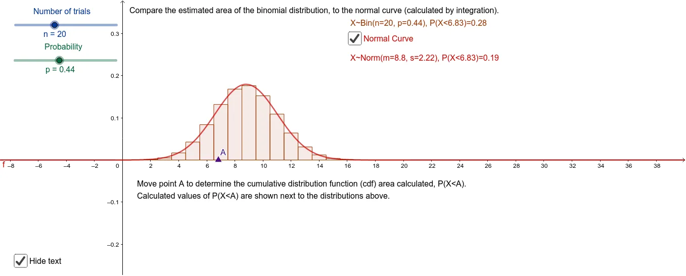
This GeoGebra example dynamically illustrates how the binomial probability mass function approximates the normal density curve as the number of trials increases. Core mathematical concepts include binomial distribution, normal distribution, central limit theorem, and the comparison between discrete probabilities and continuous densities. Construction highlights: the BinomialDist command generates the bar chart for the binomial distribution, the Normal command plots the normal curve, sliders n and p adjust parameters, and Point, Integral, and text objects annotate key values and areas. Suitable for high school or introductory college statistics courses to demonstrate the convergence of binomial to normal and to verify approximation conditions such as np and n(1-p) both greater than 5.