Comparing t-Distribution and Normal Distribution

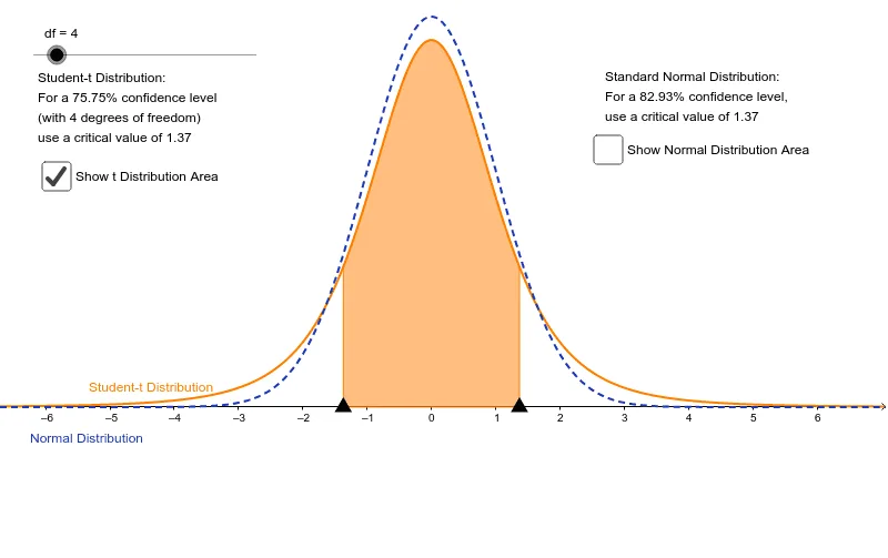
This example demonstrates the comparison of the shapes of the t-distribution and the Normal distribution by adjusting the degrees of freedom. Key math concepts include probability & statistics, distribution shapes, and critical values. It is constructed using GeoGebra commands like Point, DynamicCoordinates, and Integral, with objects such as df (degrees of freedom), A (point), f (function), B (point), a (value), C (point), D (point), g (function), b (value), aa (text), ab (text), text1 (text), text2 (text), c (value), and d (value). Suitable for high school and above students to understand statistical distribution properties and parameter effects.