
Company Employee Growth Model
Loading the math board and drawing, please wait…
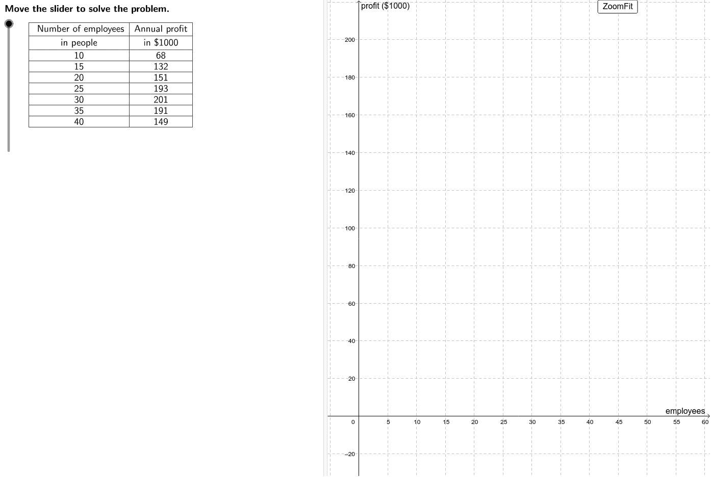
This example demonstrates the scatter plot of company employee growth over time with a logarithmic trend line. It involves core mathematical concepts like logarithmic functions, scatter plot creation, and optimal employee calculation. Key GeoGebra commands and objects used in construction include Intersect, LaTeX, Corner, TableText, Max, and If. Suitable for high school and above mathematics education, focusing on probability & statistics and optimization problems.
GeoGebra Commands & Parameters
Intersect(f, xAxis) → minEmp, maxEmpLaTeX(steps) → counterLaTeX("\text{Move the slider to solve the problem.}") → text0Corner(1) → ACorner(3) → BTableText({{LaTeX["\text{ Number of employees}"], LaTeX["\text{in people}"], A2, A3, A4, A5, A6, A7, A8}, {LaTeX["\text{Annual profit}"], LaTeX["\text{in \$1000}"], B2, B3, B4, B5, B6, B7, B8}}, "_|cv") → dataLaTeX(data) → ProblemMax({B2, B3, B4, B5, B6, B7, B8}) → maxProfitLaTeX("\text{Create a scatter plot of the data.}") → text1If(set ≟ 1, (A6, B6), If[set ≟ 2, (A5, B5), (A4, B4)]) → vertexLaTeX("\text{Vertex form of a quadratic function}") → text6LaTeX("\textcolor{#006633}{y–k=a(x–h)^2}") → text7LaTeX((((("\textcolor{#006633}{y–" * y(vertex)) * "=a(x–(") * x(vertex)) * "))^2}")) → text9LaTeX((((((((("\textcolor{#006633}{" * B2) * "–") * y(vertex)) * "=a(") * A2) * "–(") * x(vertex)) * "))^2}")) → text11LaTeX((((((((("\textcolor{#006633}{" * B2) * "–") * y(vertex)) * "=a(") * A2) * "–(") * x(vertex)) * "))^2}")) → text12LaTeX("\text{Simplify.}") → text13LaTeX((((("\textcolor{#006633}{" * LHS) * "=a(") * RHS) * ")}")) → text14LaTeX((("\text{Divide by }\textcolor{#006633}{" * RHS) * "}.")) → text15LaTeX((((("\textcolor{#006633}{a=\frac{" * LHS) * "}{") * RHS) * "}}")) → text16LaTeX("\text{Simplify.}") → text17LaTeX((("\textcolor{#006633}{a=" * a) * "}")) → text18LaTeX("\textcolor{#006633}{y–k=a(x–h)^2}") → text21LaTeX("\text{Substitute.}") → text22LaTeX((((((("\textcolor{#006633}{y-" * y(vertex)) * "=") * a) * "(x-(") * x(vertex)) * "))^2}")) → text23LaTeX((((((("\textcolor{#006633}{y-" * y(vertex)) * "=") * a) * "(x-(") * x(vertex)) * "))^2}")) → text24LaTeX("\text{Expand the squared term.}") → text25LaTeX((((((((("\textcolor{#006633}{y-" * y(vertex)) * "=") * a) * "(x^2-") * twiceVertex) * "x+") * vertsq) * ")}")) → text26LaTeX((("\text{Distribute }\textcolor{#006633}{" * a) * "}.")) → text27LaTeX((((((((("\textcolor{#006633}{y-" * y(vertex)) * "=") * a) * "x^2+(") * b) * ")x+(") * avertsq) * ")}")) → text28LaTeX((("\text{Add }\textcolor{#006633}{" * y(vertex)) * "}\text{ to both sides.}")) → text29LaTeX((((((("\textcolor{#006633}{y=" * a) * "x^2 + (") * b) * ")x + (") * c) * ")}")) → text30LaTeX((((((("\text{An equation modeling the given data is }\cr\textcolor{#006633}{y=" * a) * "x^2 + (") * b) * ")x + (") * c) * ")}.")) → text31LaTeX("\text{Graph this equation on the same graph as the scatter}\cr\text{plot to see if it is a good fit.}") → text32LaTeX("\text{This equation appears to be a good fit for the data}\cr\text{because it approximates the shape of the curve}\cr\text{suggested by the scatter plot, with points above,}\cr\text{below, and directly on the curve.}") → text33LaTeX((("\text{Substitute the point that appears to }\cr\text{be the vertex, }\textcolor{#CC0000}{" * vertex) * "}\text{, for }\textcolor{#006633}{(h, k)}. ")) → text8LaTeX((("\text{Substitute another point, the first}\cr\text{one, }\textcolor{#CC0000}{" * otherpt) * "},\text{ is convenient, for }\textcolor{#006633}{(x,y).}")) → text10LaTeX("\text{Use the vertex to determine an equation that models this data.}") → text5LaTeX("\text{Vertex form}") → text20LaTeX((((("\text{To write the equation of the parabola, substitute }\textcolor{#CC0000}{" * vertex) * "}\text{ for }\textcolor{#006633}{(h, k)}\cr\text{and substitute }\textcolor{#006633}{") * a) * "}\text{ for }\textcolor{#006633}{a}\text{ into the vertex form of a quadratic }\cr\text{function. Then simplify. }")) → text19LaTeX("\text{Assuming the profitability of this company really depends solely }\cr\text{on the number of employees, an unikely state of affairs, use the }\cr\text{model to predict the minimum and maximum number of employees }\cr\text{the company can have without losing money.}") → text34LaTeX("\text{Use the graph of the model function to approximate the zeros }\cr\text{of the function.}") → text35LaTeX((((("\text{This model suggests that the company is only profitable when it }\cr\text{has between }\textcolor{#006633}{" * lowest) * "}\text{ and }\textcolor{#006633}{") * highest) * "}\text{ employees. Note that the minimum should}\cr\text{be rounded up to the nearest whole person while the maximum }\cr\text{number should be rounded down. This ensures that profit in each }\cr\text{case is greater than or equal to zero.")) → text36LaTeX("\text{Use the buttons below to return to the original problem or randomly }\cr\text{generate a similar practice problem.}") → RandomizationTextLaTeX("\text{Let the x-axis represent the number of employees and the y-axis}\cr\text{ represent the company’s annual profit.}") → text2LaTeX("\text{Use the scatter plot to determine the type of model that represents }\cr\text{this data.}") → text3LaTeX("\text{The points in the scatter plot appear to form the shape of a }\cr\text{parabola.Therefore, the model will be in the form of a quadratic }\cr\text{function: }\textcolor{#006633}{f(x) = ax^2 + bx + c}\text{. We can find an equation to model }\cr\text{this parabola algebraically by using the vertex of the quadratic.}") → text4
AI Drawing Prompt Reference
Plot the relationship between a company's number of employees and its annual profit. Start by creating a scatter plot to represent the data points of employee numbers and annual profits. Then, use the vertex of the scatter plot to construct a vertex form quadratic function model. Predict the minimum and maximum number of employees for the company to remain profitable using the model, and mark these values on the graph. Finally, add a logarithmic trend line based on the shape of the scatter plot to better illustrate the data's trend.
The prompt above was compiled from the original drawing commands and is for reference only.