
Classic Open Box Optimization Visualization
Loading the math board and drawing, please wait…
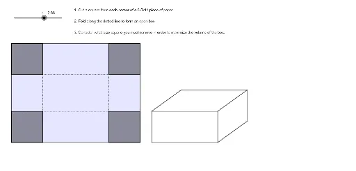
This example provides a dynamic visualization of a classic optimization problem, demonstrating how adjusting the dimensions of a rectangle maximizes the volume of an open-top box. It involves core math concepts like calculus optimization, quadratic functions, plane geometry, and 3D vectors. The construction uses GeoGebra commands such as Polygon, Point, Segment, Rotate, Line, and Intersect. Ideal for high school students and learners needing to understand optimization problems.
GeoGebra Commands & Parameters
Polygon(A, B, D, C) → q1, a, b, d, c_1Point(Circle[C, c]) → ESegment(C, E) → fPolygon(E, C, 4) → poly1, g, h, i, j, F, GPoint(Circle[A, c]) → HSegment(A, H) → kPolygon(A, H, 4) → poly2, l, m, n, p, I, JPolygon(K, B, 4) → poly3, q, r, s, t, L, MPolygon(N, D, 4) → poly4, e, f_1, g_1, h_1, O, PSegment(G, P) → i_1Segment(P, M) → j_1Segment(M, J) → k_1Segment(I, G) → l_1Point(Circle[S, 8.5 - (2 * c)]) → USegment(S, U) → m_1Rotate(U, 45°, S) → U'Segment(S, Q) → n_1Segment(Q, R) → p_1Segment(R, T) → q_1Segment(T, S) → r_1Segment(S, U') → s_1Line(U', r_1) → t_1Line(T, s_1) → a_1Line(R, s_1) → b_1Intersect(t_1, a_1) → VLine(V, q_1) → d_1Intersect(b_1, d_1) → WSegment(U', V) → e_1Segment(V, T) → f_2Segment(V, W) → g_2Segment(W, R) → h_2