
Central Limit Theorem on Tossing a Fair Die
Loading the math board and drawing, please wait…
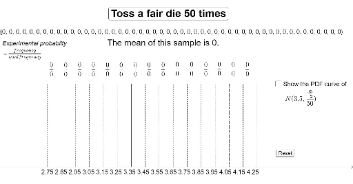
This example demonstrates the Central Limit Theorem by showing how the distribution of sample means approaches a normal distribution as the number of dice rolls increases. Key math concepts include the Central Limit Theorem, Normal Distribution, Binomial Distribution, Standard Deviation, and Integral Calculus. It is constructed using GeoGebra commands like mean, Polygon, Normal, and Integral. Suitable for high school and above students learning probability and statistics.
GeoGebra Commands & Parameters
mean(a) → bPolygon((2.75, (10 * b1 / total)), (2.75, 0), (2.85, 0), (2.85, (10 * b1 / total))) → A1, f, g, h, j_3Polygon((2.95, (10 * b3 / total)), (2.95, 0), (3.05, 0), (3.05, (10 * b3 / total))) → A3, m, n, p, qPolygon((3.05, (10 * b4 / total)), (3.05, 0), (3.15, 0), (3.15, (10 * b4 / total))) → A4, r, s, t, cPolygon((3.15, (10 * b5 / total)), (3.15, 0), (3.25, 0), (3.25, (10 * b5 / total))) → A5, d, e, f_1, g_1Polygon((3.25, (10 * b6 / total)), (3.25, 0), (3.35, 0), (3.35, (10 * b6 / total))) → A6, h_1, i_1, j_1, k_1Polygon((3.35, (10 * b7 / total)), (3.35, 0), (3.45, 0), (3.45, (10 * b7 / total))) → A7, l_1, m_1, n_1, p_1Polygon((3.45, (10 * b8 / total)), (3.45, 0), (3.55, 0), (3.55, (10 * b8 / total))) → A8, q_1, r_1, s_1, t_1Polygon((3.55, (10 * b9 / total)), (3.55, 0), (3.65, 0), (3.65, (10 * b9 / total))) → A9, a_1, b_1, c_1, d_1Polygon((3.65, (10 * b10 / total)), (3.65, 0), (3.75, 0), (3.75, (10 * b10 / total))) → A10, e_1, f_2, g_2, h_2Polygon((3.75, (10 * b11 / total)), (3.75, 0), (3.85, 0), (3.85, (10 * b11 / total))) → A11, i_2, j_2, k_2, l_2Polygon((3.85, (10 * b12 / total)), (3.85, 0), (3.95, 0), (3.95, (10 * b12 / total))) → A12, m_2, n_2, p_2, q_2Polygon((3.95, (10 * b13 / total)), (3.95, 0), (4.05, 0), (4.05, (10 * b13 / total))) → A13, r_2, s_2, t_2, a_2Polygon((4.05, (10 * b14 / total)), (4.05, 0), (4.15, 0), (4.15, (10 * b14 / total))) → A14, b_2, c_2, d_2, e_2Polygon((4.15, (10 * b15 / total)), (4.15, 0), (4.25, 0), (4.25, (10 * b15 / total))) → A15, f_3, g_3, h_3, i_3Polygon((2.85, (10 * b2 / total)), (2.85, 0), (2.95, 0), (2.95, (10 * b2 / total))) → A2, i, j, k, lNormal(3.5, sqrt(35 / 600), x, false) → p_3Integral(p_3, 2.75, 4.25) → u
AI Drawing Prompt Reference
Create a diagram illustrating the Central Limit Theorem for a fair die, showing how the distribution of sample means approaches a normal distribution as the number of throws increases. First, calculate the mean of each throw, then draw rectangles to represent the frequency distribution of different means, followed by a normal distribution curve, and finally use integration to calculate the area under the curve.
The prompt above was compiled from the original drawing commands and is for reference only.