Central Limit Theorem for Samples from a Binomial Distribution

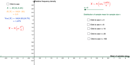
This GeoGebra example demonstrates the central limit theorem by comparing the distribution of sample means or sums drawn from a binomial distribution with a normal distribution. It highlights binomial probability, random sampling, sample size, success probability, mean, standard deviation, and convergence to normality. The construction uses Histogram to display the empirical distribution of repeated samples, Normal to overlay the theoretical normal curve, and BinomialDist to model the underlying binomial experiment. Labeled points and input objects such as A, B, D, E, G, H, J, K, M, and N likely control trial count, probability, sample size, bin width, and displayed statistics. It is suitable for high school probability extensions, introductory college probability and statistics, and classroom simulations of sampling distributions.