
Bouncing Ball Model
Loading the math board and drawing, please wait…
In collections
Physics Lab
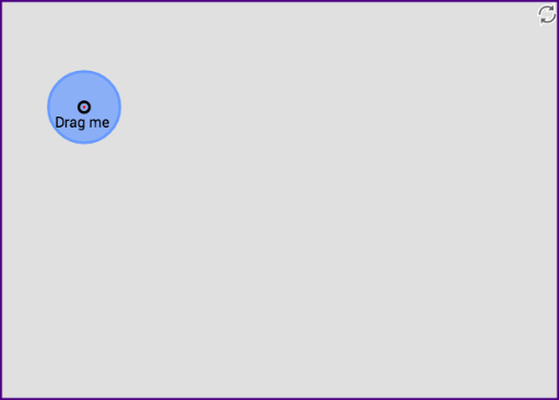
This example demonstrates the motion trajectory and collision effects of a bouncing ball under gravity. It involves core mathematical concepts like vectors, transformations, coordinate geometry, parametric equations, and function graphing. Key construction elements include Circle, Vector, Ray, Segment, OrthogonalLine, If, Mirror, and Slider commands/objects in GeoGebra. Suitable for high school students studying physical motion laws, spatial geometric transformations, and mathematical modeling.
GeoGebra Commands & Parameters
Circle(A, m1 / 2) → cVector(A, A') → vi1Ray(A, A') → fSegment((x(Corner[4]), y(Corner[4])), (x(Corner[3]), y(Corner[3]))) → hSegment((x(Corner[4]), y(Corner[4])), (x(Corner[1]), y(Corner[1]))) → iSegment((x(Corner[2]), y(Corner[2])), (x(Corner[3]), y(Corner[3]))) → jSegment((x(Corner[1]), y(Corner[1])), (x(Corner[2]), y(Corner[2]))) → kOrthogonalLine(A, xAxis) → lOrthogonalLine(A, l) → mIf(x(A) > xmax - m1 / 2, 0, If[x(A) < xmin + m1 / 2, 1, If[y(A) < ymin + m1 / 2, 2, If[y(A) > ymax - m1 / 2, 3, 4]]]) → collisionMirror(A', l) → A''Mirror(A', m) → A''_1