
Biscribed Snub Cube (laevo) n=24: Polyhedra with Extreme Distribution of Equival
Loading the math board and drawing, please wait…
In collections
₈Polyhedra with extreme distribution of equivalent vertices
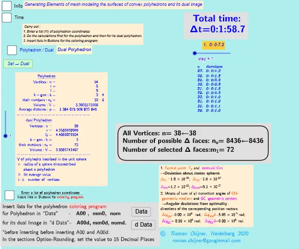
① This example demonstrates a biscribed snub cube (laevo configuration) with 24 equivalent vertices, belonging to a class of polyhedra that achieve extreme distributions of vertices (e.g., minimizing or maximizing certain metrics). ② Core mathematical concepts include polyhedral geometry, vertex equivalence, extreme distributions, circumscribed and inscribed spheres (biscribed property), and optimization problems (such as linear programming or geometric mean). ③ Construction highlights: from the construction summary, GeoGebra commands such as Sequence, Element, Div, Sum, If, and Text are used, along with objects like sphere volume (Volsphere), radius (r), vertex coordinates (A00), and a button (button3) for interaction, likely controlling the parameter n to update vertex count and dynamically compute volumes and radii. ④ Suitable for high school to university-level teaching of solid geometry, polyhedra, and optimization topics, as well as for mathematical modeling or computer-aided geometric design demonstrations.
GeoGebra Commands & Parameters
Text("" + p) → txt_pSum(Flatten[Sequence[Append[Sequence[Element[txt_p, i], i, m01(k), m02(k)], " "], k, 1, 5]]) → txtUm1If(bu0, A00, A00d) → A00_0Length(A00_0) → nLength(l2) → läl2Sequence(sgn(Determinant[{Element[A00_0, i1] - Element[A00_0, j], Element[A00_0, i2] - Element[A00_0, j], Element[A00_0, i3] - Element[A00_0, j]}]), j, 1, n) → l01Length(A00d) → zzzSum(Zip[(T * F), T, SysTimeAkt1, F, {1, 1000, 60000, 3600000, 86400000}]) → TimeAbs1Sum(Zip[(T * F), T, SysTimeAkt2, F, {1, 1000, 60000, 3600000, 86400000}]) → TimeAbs2Div(TimeRelab, 3600) → HDiv(TimeRelab - (H * 3600), 60) → MElement(ZwZeit, step) → text10TableText({Append["a duration", Last[ZwZeit, Min[10, Length[ZwZeit]]]]}, "v") → text2cLength(A00) → lm1If(Length[Unique[l01 \ {0}]] ≟ 1, 7, -7) → a7Sum(Zip[(T * F), T, SysTimeAkt0, F, {1, 1000, 60000, 3600000, 86400000}]) → TimeAbs0Div(TimeRelab0, 3600) → H0Div(TimeRelab0 - (H0 * 3600), 60) → M0Text("" + (TimeRelab0 - (H0 * 3600) - (M0 * 60))) → S0aText("" + (TimeRelab - (H * 3600) - (M * 60))) → SIndexOf(".", S) → indexIndexOf(".", S0a) → indexaFirst(S, index + 1) → txtSFirst(S0a, indexa + 1) → txtS0aIf(bu0, " ", "d") → txtbuoMax(Length[A00], Length[A00d]) → maxläElement(A00, 24) → m11TableText({{"\underline{Polyhedron}"}, Append["Vertices: n=", {Length[A00]}], Append["r=", {r}], Append["\bar{r}=", {r_m}], Append["k-gon : k=", mm5a], Append["their\; numbers: n_k=", mm7a], Append["Volume: V=", {Vol_r}], Append["Average\; distance: p=", {txtUm1}]}, "hr ") → text7TableText({{"\underline{dual\;Polyhedron}"}, Append["Vertices: n=", {Length[A00d]}], Append["r=", {r_d}], Append[" \bar{r_d}= ", {r_md}], Append["k-gon : k=", mm5ad], Append["their\; numbers: n_k=", mm7ad], Append["Volume: V=", {Vold_r}]}, "hr ") → text20
AI Drawing Prompt Reference
Draw a biscribed snub cube with 24 equivalent vertices, showing an extreme distribution of vertex positions. Include both circumscribed and inscribed spheres, and label key data such as vertex count, sphere radii, average vertex distance from center, and volume. Start by defining vertex positions, then draw the spheres, and finally add the labels.
The prompt above was compiled from the original drawing commands and is for reference only.