
Binomial Distribution Simulation by Heather Pierce
Loading the math board and drawing, please wait…
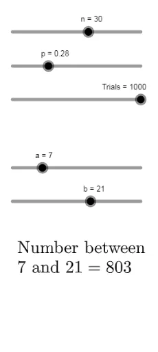
This example demonstrates the binomial distribution random phenomenon. The core math concepts involved are binomial distribution in probability & statistics. Construction highlights include using GeoGebra commands Sequence, Sort, Max, CountIf and objects t, n, p, t_1, p_1, n_1, list, sorted, heights, Points1, Points2, l1, h, a, b, num, text1. Suitable for high school and above students learning probability statistics and discrete mathematics.
GeoGebra Commands & Parameters
Sequence(RandomBinomial[n, p], i, 1, t, 1) → listSort(list) → sortedSequence(CountIf[x ≟ i, sorted], i, 0, n, 1) → heightsSequence((i - 0.5, Element[heights, i + 1]), i, 0, n, 1) → Points1Sequence((i + 0.5, Element[heights, i + 1]), i, 0, n, 1) → Points2Sequence(Polygon[(i - 0.5, 0), (i + 0.5, 0), Element[Points2, i + 1], Element[Points1, i + 1]], i, 0, n - 1, 1) → l1Max(Sequence[y(Element[Points1, i]), i, 1, Length[Points1]]) → hCountIf(a ≤ x ∧ x ≤ b, sorted) → num
AI Drawing Prompt Reference
Create a graph demonstrating the binomial distribution phenomenon, featuring a probability function with sliders for parameters. Generate random binomial distribution data using sequences, sort the data, and calculate frequencies for each value. Represent the frequency distribution as a bar chart, where each bar is formed by two points, with the base on the x-axis and height corresponding to frequency, showcasing the characteristic shape of the binomial distribution.
The prompt above was compiled from the original drawing commands and is for reference only.