
Binomial and Poisson Distributions
Loading the math board and drawing, please wait…
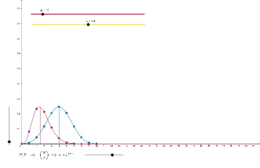
This example demonstrates the graphical characteristics and core mathematical concepts of the binomial and Poisson distributions. By adjusting parameters n and p, the probability distribution graph of the binomial distribution can be observed. Meanwhile, by changing parameter λ, the probability distribution graph of the Poisson distribution can be observed. The construction summary uses GeoGebra commands such as Sequence and Segment, suitable for high school and above students to learn probability and statistics.
GeoGebra Commands & Parameters
Sequence(((nCr[n, r] * p^(r)) * (1 - p)^(n - r)), r, 0, n) → BSequence(k, k, 0, n) → XSequence(((ℯ^((-m)) * s^(m))) / s!, s, 0, n) → PoSegment(((n * p), 0), ((n * p), b((n * p)))) → EBSegment((m, 0), (m, po(m))) → EPo
AI Drawing Prompt Reference
Plot the probability distribution graphs of binomial and Poisson distributions. First, adjust parameters n and p to observe the binomial distribution graph. Then, change parameter λ to observe the Poisson distribution graph. Use the sequence command to generate the probability value sequence B for the binomial distribution and the x-axis value sequence X, and generate the probability value sequence Po for the Poisson distribution. Finally, draw the cumulative probability segment EB for the binomial distribution and the cumulative probability segment EPo for the Poisson distribution.
The prompt above was compiled from the original drawing commands and is for reference only.