
Area Under a Linear Function
Loading the math board and drawing, please wait…
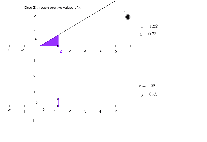
This example demonstrates how the area under a linear function changes by graphing the values of the area. Key mathematical concepts include functions, geometric construction, and integration. GeoGebra commands used include Point, Line, OrthogonalLine, Intersect, Circle, Ray, Polygon, Segment, and more. Suitable for middle school and above students to learn about function graphs and integration.
GeoGebra Commands & Parameters
Point(yAxis) → APoint(yAxis) → BPoint(yAxis) → CPoint(xAxis) → DPoint(xAxis) → EPoint(xAxis) → FPoint(xAxis) → GPoint(xAxis) → HPoint(xAxis) → IPoint(yAxis) → KPoint(yAxis) → LPoint(yAxis) → MLine(M, xAxis) → aOrthogonalLine(M, a) → bLine(E, J) → cPoint(b) → NPoint(b) → OPoint(a) → PPoint(a) → QPoint(a) → RPoint(a) → SPoint(a) → TPoint(a) → UPoint(a) → VPoint(a) → WLine(B, K) → dLine(A, O) → ePoint(a) → ZOrthogonalLine(Z, c) → fIntersect(c, f) → A_1Circle(Z, (m * x(Z))) → gIntersect(g, f) → B_1, C_1Ray(M, C_1) → hPolygon(M, Z, C_1) → poly1, c_1, m_1, zCircle(A_1, ((m * x(B)) * x(b) / 2)) → kCircle(A_1, ((m * x(Z)) * x(Z) / 2)) → pIntersect(p, f) → D_1, E_1Segment(E_1, A_1) → iSegment(B, K) → jSegment(A, O) → l