
Animation 248: Composite Construction of Triangle Incircle, Circumcircle, Rotati
Loading the math board and drawing, please wait…
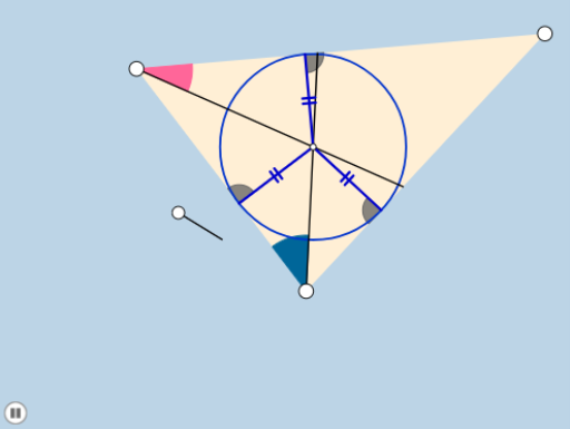
① This example demonstrates a dynamic geometric animation involving a triangle, its circumcircle, incircle, and composite transformations (rotation and dilation), with sliders controlling parameters to observe how the figure changes with angles or scale factors. ② Core mathematical concepts include the incenter, circumcenter, incircle, circumcircle, similarity and homothety (dilation), rotational symmetry, angle relationships, right triangle properties, and the integration of scatter plots with arithmetic operations, reflecting the fusion of geometry and algebra. ③ Construction highlights: Based on the construction summary, GeoGebra commands such as Line, Slope, PointIn, Angle, Segment, Min, Circle, Intersect, Incircle, Center, Polygon, Rotate, Ray, CircleSector, Dilate, OrthogonalLine, CircleArc, and LineBisector are used, creating objects A, B, d, m, b, a, c, C, e, f, α, β, γ, g, h, i, list1, j, q, p, k, D, E, F, G, H, I_2, J, K, L, N, O, P, δ, ε, η, θ, r, inc, and I. Sliders drive rotation and scaling, updating the figure dynamically. ④ Suitable for high school to early college geometry instruction, for exploring triangle centers, circle properties, and composite transformations, and as a dynamic geometry courseware or mathematical experiment material.
GeoGebra Commands & Parameters
Line(A, B) → dSlope(d) → aPointIn(c) → CLine(A, C) → eLine(B, C) → fAngle(B, A, C) → αAngle(A, C, B) → βAngle(C, B, A) → γSegment(A, C) → gSegment(C, B) → hSegment(B, A) → iMin(list1) → jCircle(C, (0.2 * j)) → qCircle(A, (0.2 * j)) → pCircle(B, (0.2 * j)) → kIntersect(q, f, 2) → DIntersect(q, e, 1) → EIntersect(q, e, 2) → FIntersect(p, e, 2) → GIntersect(p, d, 1) → HIntersect(k, f, 2) → I_2Intersect(k, d, 2) → JIntersect(d, i) → KIntersect(d, i) → LIntersect(k, f, 1) → NIntersect(p, e, 1) → OIntersect(p, d, 2) → PAngle(D, C, E) → δAngle(O, A, P) → εAngle(J, B, I_2) → ηAngle(G, A, H) → θIncircle(A, B, C) → rCenter(r) → ILine(C, I) → lLine(A, I) → nLine(B, I) → sIntersect(e, s) → RIntersect(d, l) → SIntersect(f, n) → TPolygon(A, B, C) → poly1, c_1, a_1, b_1Rotate(D, δ / 2, C) → D'Angle(D, C, D') → κRotate(J, η / 2, B) → J'Angle(J, B, J') → λRay(C, D') → tRay(B, J') → e_1Rotate(O, ε / 2, A) → O'Angle(O, A, O') → ιRay(A, O') → d_1Segment(C, S) → f_1Segment(A, T) → g_1Segment(B, R) → h_1Intersect(q, f_1, 1) → UIntersect(q, f, 1) → VIntersect(p, g_1, 1) → WIntersect(k, h_1, 1) → ZCircleSector(A, P, W) → q_1CircleSector(B, I_2, Z) → p_1Dilate(C, If[0 < m ≤ 1, 1 - m, 0], S) → C'Dilate(B, If[2 < m ≤ 3, 3 - m, 0], R) → B'Segment(B, B') → j_1Rotate(p_1, If[3 < m ≤ 4, ((m - 3) * γ / 2), γ / 2], B) → s_1Dilate(A, If[4 < m ≤ 5, 5 - m, 0], T) → A'Segment(A, A') → l_1Rotate(q_1, If[5 < m ≤ 6, ((m - 5) * α / 2), α / 2], A) → t_1OrthogonalLine(I, f) → m_1OrthogonalLine(I, d) → n_1OrthogonalLine(I, e) → a_2Intersect(f, m_1) → MIntersect(d, n_1) → A_1Intersect(e, a_2) → B_1Segment(I, M) → b_2Circle(M, (0.2 * b_2)) → c_2Intersect(c_2, f, 1) → C_1Intersect(c_2, b_2, 1) → D_1Intersect(c_2, f, 2) → E_1CircleSector(M, E_1, D_1) → d_2Dilate(I, If[6 < m ≤ 7, 7 - m, 0], M) → Q'Segment(I, Q') → e_2Rotate(d_2, If[7.5 < m ≤ 8.5, ((m - 7.5) * π / 2), 1.5707963267948966], M) → f_2Segment(I, B_1) → g_2Segment(I, A_1) → h_2Circle(B_1, (0.2 * g_2)) → k_2Circle(A_1, (0.2 * h_2)) → p_2Intersect(k_2, e, 2) → F_1Intersect(k_2, g_2, 1) → G_1Intersect(k_2, e, 1) → H_1Intersect(p_2, d, 2) → I_1Intersect(p_2, h_2, 1) → J_1Intersect(p_2, d, 1) → K_1Dilate(I, If[8.5 < m ≤ 9.5, 9.5 - m, 0], B_1) → Q'_1Segment(I, Q'_1) → i_2CircleSector(B_1, H_1, G_1) → q_2CircleSector(A_1, I_1, J_1) → r_2Rotate(q_2, If[10 < m ≤ 11, ((m - 10) * π / 2), 1.5707963267948966], B_1) → s_2Dilate(I, If[11 < m ≤ 12, 12 - m, 0], A_1) → Q'_2Segment(I, Q'_2) → j_2Rotate(r_2, If[12.5 < m ≤ 13.5, ((m - 12.5) * π / 2), 1.5708], A_1) → t_2Angle(M, I, B_1) → ζAngle(B_1, I, A_1) → μAngle(A_1, I, M) → νRotate(I, If[14 < m ≤ 15, ((m - 14) * ζ), ζ], I) → Q'_3Rotate(Q', If[14 < m ≤ 15, ((m - 14) * ζ), ζ], I) → Q''Segment(Q'_3, Q'') → l_2Rotate(Q'_3, If[15 < m ≤ 16, ((m - 15) * μ), μ], I) → L_1Rotate(Q'', If[15 < m ≤ 16, ((m - 15) * μ), μ], I) → Q'''Segment(L_1, Q''') → m_2Rotate(A_1, If[16 < m ≤ 18, ((m - 16) * π), 6.28319], I) → M'Intersect(m_1, f) → QCircle(I, Q) → d_3Line(A, B) → n_2CircleArc(I, A_1, M') → c_3Circle(A, I, B) → k_1LineBisector(I, B) → i_1LineBisector(I, A) → r_1Intersect(i_1, r_1) → M_1Dilate(M_1, If[19 < m ≤ 20, 20 - m, 0], B) → N_1Segment(M_1, N_1) → f_3Rotate(B, If[20 < m ≤ 22, ((m - 20) * π), (2 * π)], M_1) → B'_1CircleArc(M_1, B, B'_1) → e_3Dilate(C, If[22 < m ≤ 23, 23 - m, 0], I) → C'_1Segment(C, C'_1) → g_3Dilate(I, If[23 < m ≤ 24, 24 - m, 0], M_1) → I'Segment(I, I') → h_3
AI Drawing Prompt Reference
Create a dynamic geometric animation showing a triangle, its circumcircle, and incircle, with sliders controlling rotation and scaling parameters to observe how the figure changes with angles or scale factors. The animation includes triangle centers, circle properties, similarity and homothety (dilation), rotational symmetry, angle relationships, right triangle properties, and the integration of geometry and algebra, such as scatter plots with arithmetic operations.
The prompt above was compiled from the original drawing commands and is for reference only.