
Analysis of the Normal Curve
Loading the math board and drawing, please wait…
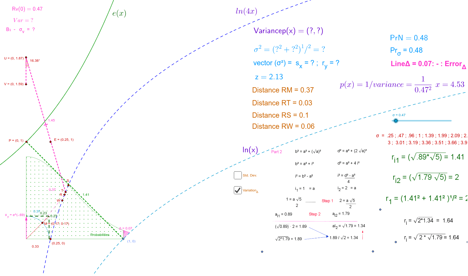
This example demonstrates the geometric analysis of the normal curve. Key mathematical concepts include probability distribution, function graphing, and geometric transformations. Construction involves commands like Integral, Vector, Point, CircleArc, Intersect, Angle, Polygon, Distance, and Translate. Suitable for high school students or college undergraduates to understand the geometric significance and applications of the normal curve.
GeoGebra Commands & Parameters
Integral(f, 0, 1) → pr_NIntegral(g, 0, 0.851) → Area_σName(Area_σ) → C1Name(pr_N) → A1Name(pr_σ) → B1Vector((0.5015760690660556, 0)) → uVector((0, 0.5015760690660556)) → vVector((0.5015760690660556, 0.5015760690660556)) → wPoint(c_v) → APoint(h) → DPoint(d) → BSegment(B, D) → aSegment(D, A) → bCircleArc(C, B, A) → cIntegral(g(x) / σ, 0, 0.851) → RvSegment(C, D) → i_2Segment(B, A) → jName(k) → D1Intersect(p, a, 1) → σ_∨Segment(C, σ_∨) → lAngle(σ_∨, C, D) → αIntersect(f, f_1, (1.066731473723258, 0.06459927655136193)) → FPoint(f) → GSegment(G, F) → ΔPoint(f_1) → HPoint(f_1) → IPoint(f_1) → JPoint(f_1) → KPolygon(F, I, J, K, H, G) → poly1, f_2, i_1, j_1, k_1, h_1, g_2Point(p_1) → LPoint(i_2) → MPoint(c) → NPoint(c) → OPoint(g_1) → PSegment(σ_∨, M) → e_ePoint(p_1) → RSegment(R, M) → a_1Point(p_1) → SDistance(R, S) → distanceRSDistance(R, M) → distanceRMIntersect(pr_N, p_1, (0.40536109480235216, 0.48331734052759795)) → TDistance(R, T) → distanceRTDistance(R, σ_∨) → distanceRσ∨Segment(R, σ_∨) → b_1Point(p_1) → WDistance(R, W) → distanceRWDistance(S, E) → distanceSEDistance(T, E) → distanceTEDistance(R, E) → distanceREDistance(W, E) → distanceWEDistance(W, P) → distanceWPDistance(R, P) → distanceRPDistance(T, P) → distanceTPDistance(S, P) → distanceSPDistance(T, V) → distanceTVDistance(T, U) → distanceTUSegment(T, U) → c_1Segment(U, V) → d_1Angle(V, U, T) → βVector(Z, A_1) → u_1Translate(C, u_1) → C'Translate(σ_∨, u_1) → B_1Segment(C', B_1) → l'Segment(T, B_1) → e_1Polygon(T, U, B_1) → poly2, b_2, t_1, u_2Point(e_1) → C_1Segment(Q, P) → m_1
AI Drawing Prompt Reference
Draw a normal distribution curve and its geometric analysis. Start with two curves: one standard normal curve and one transformed curve. Shade the area under the curve from zero to one and label the integral value. From the origin, draw three vectors along the x-axis, y-axis, and diagonal. Select several key points on the curves, connect them to form a polygon, and add arcs, segments, and angle marks. Include multiple auxiliary points, measure and display distances between points, and show the area between the curve and axes. The overall figure illustrates the geometric properties and transformations of the probability density function.
The prompt above was compiled from the original drawing commands and is for reference only.