Alpha, Beta, and Power in Hypothesis Testing

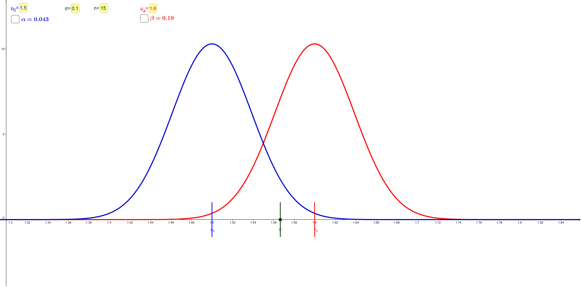
This GeoGebra example dynamically visualizes the relationship between Type I error (α), Type II error (β), and statistical power (1-β) in hypothesis testing. It uses normal distribution curves, critical regions, and sampling distributions to show how these error probabilities change with sample size, significance level, and effect size when the null and alternative means differ. Core mathematical concepts include hypothesis testing, normal distribution, significance level, power function, and the trade-off between Type I and Type II errors. Construction highlights: Point defines means, Normal generates distribution curves, OrthogonalLine creates perpendicular guides, Integral computes shaded areas representing α and β, Textfield and inputBox allow interactive parameter adjustment, and Segment connects key points. Suitable for high school or university statistics courses, this tool helps students understand decision rules and power analysis, and serves as an interactive classroom demonstration or self-study resource.