
3D Explanation of Invariance of Sum of Squares of Distances using Steiner Theore
Loading the math board and drawing, please wait…
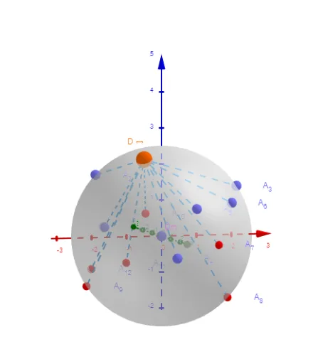
This example demonstrates the invariance of the sum of squares of distances in 3D using Steiner's theorem. Key math concepts include centroid, special points, sphere, surface, and scatter plot. GeoGebra commands used are Sphere, PointIn, Flatten, Zip, Length, RotateText, with objects like r, O, a, A1-A6, l, l1, D, l2, b, n, text1, Cm, text2, sum, text3, l4, text5, text4, text6, txt, txt1, text7. Suitable for high school and above, focusing on solid geometry and inequalities.
GeoGebra Commands & Parameters
Sphere(O, r) → aPointIn(a) → A1PointIn(a) → A2PointIn(a) → A3PointIn(a) → A4PointIn(a) → A5PointIn(a) → A6Flatten({l, (-l)}) → l1PointIn(a) → DZip(Segment[D, a], a, l1) → l2Length(l2) → nZip(Text["A_{" + (k) + "}", b + (0.5, 1)], k, Sequence[n], b, l1) → l4RotateText(txt, 90°) → txt1
AI Drawing Prompt Reference
Draw a sphere in 3D space and randomly select six points on its surface. Draw a line through the center of the sphere and extend it in both directions. Select a point on this line and connect it to the six points on the sphere's surface. Calculate the lengths of these connecting segments and label them on the line. Finally, rotate the labels 90 degrees to clearly show the relationship between the distances from the points on the sphere to the line, emphasizing the invariance of the sum of the squares of the distances.
The prompt above was compiled from the original drawing commands and is for reference only.