
三角函数图像研究 by Mathguru
几何画板及绘图内容加载中,请稍等……
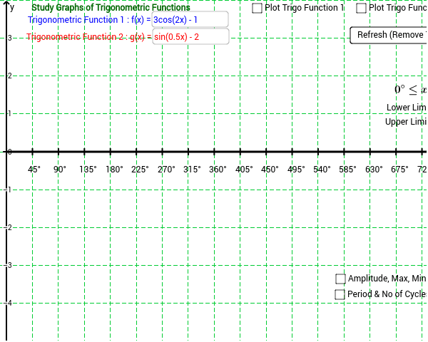
这个范例演示了如何使用 GeoGebra 绘制并研究两个三角函数的图像,包括设置上下限。涉及的核心数学概念有三角函数、几何变换、函数图像绘制。作图要点包括使用 If、Function、Derivative、RemoveUndefined、Point、Textfield、Sequence、Asymptote、Intersect、Distance、Vector、Midpoint 等命令和对象。适合高中及以上学生用于自我学习和探索三角函数的性质。
GeoGebra 命令及参数
If(angledegree, lowerlimit_d * π / 180, lowerlimit_r) → lowerlimitIf(angledegree, upperlimit_d / 180, upperlimit_r) → upperlimitFunction(g_{hidden}, lowerlimit * π, upperlimit * π) → gDerivative(g_{hidden}) → g'RemoveUndefined(Sequence[x(Root[g', i]), i, -31.41593, 31.41593, 0.31416]) → sincosturningptslistgFunction(f_{hidden}, lowerlimit * π, upperlimit * π) → fDerivative(f_{hidden}) → f'RemoveUndefined(Sequence[x(Root[f', i]), i, -31.41593, 31.41593, 0.31416]) → sincosturningptslistfPoint(g) → P_{02}Point(f) → P_{01}If(Length[sincosturningptslistg] > 0, false, true) → gchecktanfunction2Derivative(g') → g''Derivative(f') → f''If(Length[sincosturningptslistf] > 0, false, true) → fchecktanfunction1Textfield(f_{hidden}) → inputBox1Textfield(g_{hidden}) → inputBox4Sequence(Text[i + "°", (π / 180 * i - 0.05, -0.3)], i, 0, 1080, 90) → listxaxisdegreesby90If(fchecktanfunction1 ≟ false, (y(Max[f, lowerlimit * π, upperlimit * π * 10]) + y(Min[f, lowerlimit * π, upperlimit * π * 10])) / 2, meanline_{1fortan}) → meanline_1If(gchecktanfunction2 ≟ false, (y(Max[g, lowerlimit * π, upperlimit * π * 10]) + y(Min[g, lowerlimit * π, upperlimit * π * 10])) / 2, meanline_{2fortan}) → meanline_2Textfield(h_{hidden}) → inputBox5Function(h_{hidden}, lowerlimit * π, upperlimit * π) → hFunction(meanline_1, lowerlimit * π, upperlimit * π) → f_{meanline1}Function(meanline_2, lowerlimit * π, upperlimit * π) → g_{meanline2}Textfield(lowerlimit_d) → inputBox6Textfield(upperlimit_d) → inputBox7Function(0, lowerlimit * π, upperlimit * π + 1) → h_{x-axis}Textfield(upperlimit_r) → inputBox3Textfield(lowerlimit_r) → inputBox2Sequence(Text[FractionText[i] + "π", (π * i - 0.15, -0.1), true, true], i, lowerlimit + xunitdistance, upperlimit, xunitdistance) → listxaxisradianlabelSequence((i, 0), i, lowerlimit * π, upperlimit * π, xunitdistance * π) → listxaxisticksSequence(abs(f(i)), i, lowerlimit * π, upperlimit * π, 0.01) → valuestanfunctionAsymptote(f) → list5Asymptote(Function[g, lowerlimit * π, upperlimit * π]) → list6If(fchecktanfunction1 ≟ false, y(Max[f, lowerlimit * π, upperlimit * π * 10]), 0) → maxline_1If(fchecktanfunction1 ≟ false, y(Min[f, lowerlimit * π, upperlimit * π * 10]), 0) → minline_1Function(maxline_1, lowerlimit * π, upperlimit * π) → f_{maxline1}Function(minline_1, lowerlimit * π, upperlimit * π) → f_{minline1}Intersect(f_{maxline1}, vertline1) → A_1Intersect(f_{minline1}, vertline1) → B_1Intersect(f_{meanline1}, vertline1) → C_1Distance(A_1, C_1) → distanceA1C1Vector(C_1, A_1) → u_1Vector(C_1, B_1) → v_1Midpoint(A_1, C_1) → M_{A1C1}Midpoint(B_1, C_1) → M_{C1B1}If(gchecktanfunction2 ≟ false, y(Max[g, lowerlimit * π, upperlimit * π * 10]), 0) → maxline_2If(gchecktanfunction2 ≟ false, y(Min[g, lowerlimit * π, upperlimit * π * 10]), 0) → minline_2Function(maxline_2, lowerlimit * π, upperlimit * π) → g_{maxline1}Function(minline_2, lowerlimit * π, upperlimit * π) → g_{minline1}Intersect(g_{maxline1}, vertline2) → A_2Intersect(g_{minline1}, vertline2) → B_2Intersect(g_{meanline2}, vertline2) → C_2Midpoint(A_2, C_2) → M_{A2C2}Midpoint(B_2, C_2) → M_{B2C2}Distance(A_2, C_2) → distanceACVector(C_2, A_2) → u_2Vector(C_2, B_2) → v_2If(fchecktanfunction1, tancyclesf, sincoscycles1) → cycles1If(gchecktanfunction2, tancyclesg, sincoscycles2) → cycles2Intersect(g, vertline3, (0, -2)) → P_1Midpoint(P_1, Q_1) → M_{P1Q1}Vector(M_{P1Q1}, P_1) → u_{p1l}Vector(M_{P1Q1}, Q_1) → u_{p1r}Intersect(f, vertline4, (0.37243505127654164, 1.2055278889599705)) → P_2Midpoint(P_2, Q_2) → M_{P2Q2}Vector(M_{P2Q2}, Q_2) → u_{p2r}Vector(M_{P2Q2}, P_2) → u_{p2l}Derivative(f'') → f'''Derivative(g'') → g'''Sequence(Text[i + "°", (π / 180 * i - 0.15, -0.55)], i, lowerlimit * 180 + 180 * xunitdistance, upperlimit * 180, 180 * xunitdistance) → listxaxisdegreesby45
AI 绘图提示语参考
绘制两个三角函数的图像,并标出上下限范围。首先画出两个函数及其导数,然后找到导数的零点作为关键点。接着,计算并画出每条函数图像的平均线,以及最大值和最小值所在的水平线。最后,添加坐标轴、角度和弧度刻度,以及函数图像的渐近线。
以上提示语为根据原始绘图命令整理而来,仅供参考。