
P值与临界值比较
几何画板及绘图内容加载中,请稍等……
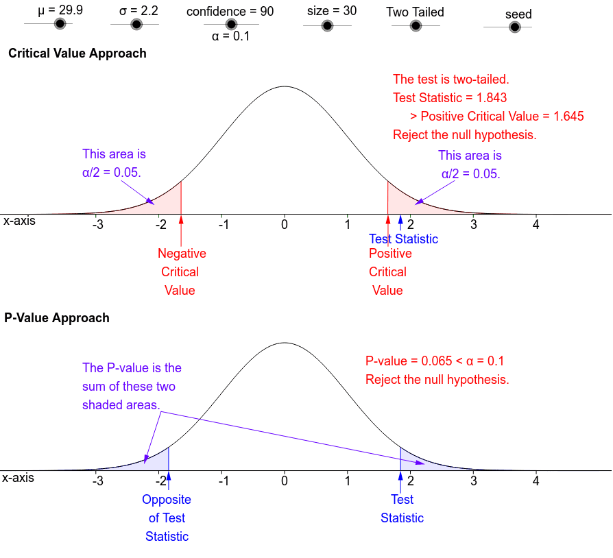
①本范例演示假设检验中临界值法与P值法的对比过程;②涉及核心数学概念包括假设检验、P值、临界值、正态分布;③作图要点:运用了Sequence, Append, Element, Mean, Integral, Line, Vector, If, IntegralBetween, Text等GeoGebra命令与对象构建正态分布曲线、样本均值、临界值与P值;④适合高中及以上数学、统计学学习者理解假设检验方法。
GeoGebra 命令及参数
Sequence(k, k, 80, 99) → CL1Append(CL1, 99.9) → CL2Element(CL2, cs) → ConfidenceSequence(RandomNormal[μ + Type - 2 + seed, σ], k, 1, size) → SampleMean(Sample) → xbarIntegral(BellCurve, TstSt, 10) → PVhiIntegral(BellCurve, -10, TstSt) → PVloLine((-5, 0), (5, 0)) → XAx2Vector(TST2, TSH2) → TSV1If(Type ≟ 2, (-InverseNormal[0, 1, α / 2]), (-InverseNormal[0, 1, α])) → CVhiVector(TST1, TSH1) → TSV2If(Type ≟ 2, InverseNormal[0, 1, α / 2], InverseNormal[0, 1, α]) → CVloVector(CVT2, CVH2) → CVVhiIntegral(exp((-x^(2))) / ((4 * 3.141592653589793)), TstSt, 10) → MhixIntegral((x * e^(((-x^(2))) / 2) / sqrt((2 * 3.141592653589793))), TstSt, 10) → MhiyVector(CVT1, CVH1) → CVVloIntegral(exp((-x^(2))) / ((4 * 3.141592653589793)), -10, TstSt) → MloxIntegral((x * e^(((-x^(2))) / 2) / sqrt((2 * 3.141592653589793))), -10, TstSt) → MloyVector(A, CMlo) → PVVloVector(B, CMhi) → PVVhiElement(TypTx, Type) → typeIntegral(exp((-x^(2))) / ((4 * 3.141592653589793)), CVhi, 10) → Mhix2Integral((x * e^(((-x^(2))) / 2) / sqrt((2 * 3.141592653589793))), CVhi, 10) → Mhiy2Vector(C, CMhi2) → AlphaRVIntegral(exp((-x^(2))) / ((4 * 3.141592653589793)), -10, CVlo) → Mlox2Integral((x * e^(((-x^(2))) / 2) / sqrt((2 * 3.141592653589793))), -10, CVlo) → Mloy2Vector(D, CMlo2) → AlphaRCMIntegral(BellCurve, -5, (-abs(TstSt))) → TTLfIntegral(BellCurve, abs(TstSt), 5) → TTRtIntegral(exp((-x^(2))) / ((4 * 3.141592653589793)), -10, (-abs(TstSt))) → Mlox3Integral((x * e^(((-x^(2))) / 2) / sqrt((2 * 3.141592653589793))), -10, (-abs(TstSt))) → Mloy3Integral(BellCurve, -10, (-abs(TstSt))) → MTTLIntegral(exp((-x^(2))) / ((4 * 3.141592653589793)), abs(TstSt), 10) → Mhix3Integral((x * e^(((-x^(2))) / 2) / sqrt((2 * 3.141592653589793))), abs(TstSt), 10) → Mhiy3Vector(E, CMlo3) → TTLVVector(E, CMhi3) → vVector(F, CMlo4) → AHLVVector(G, CMhi4) → AHHVVector(OTSLP, OTSP) → uSequence(Segment[(k, (-0.01)), (k, 0)], k, -3, 4) → XTcSq2Sequence(Text[k, (k - 0.05, (-0.045))], k, -3, 4) → XLbTxSq2Line((-5, 0.8), (5, 0.8)) → XAx1Sequence(Segment[(k, 0.79), (k, 0.8)], k, -3, 4) → XTcSq1Sequence(Text[k, (k - 0.05, 0.755)], k, -3, 4) → XLbTxSq1IntegralBetween(BellCurve2, 0.8, CVhi, 4.5) → AlFlRtIntegralBetween(BellCurve2, 0.8, -5, CVlo) → AlFlLfIntegralBetween(BellCurve2, 0.8, -5, CVlo) → AlHfLfIntegralBetween(BellCurve2, 0.8, CVhi, 4.5) → AlHfRtText("Test Statistic", (TstSt - 0.5, 0.71)) → TSLab2