
Picard–Lindelöf迭代:当h(x,y)与h_y(x,y)处处有界连续时解全局存在
几何画板及绘图内容加载中,请稍等……
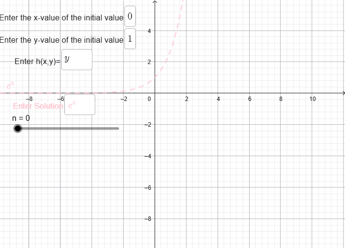
该范例通过GeoGebra动态演示Picard–Lindelöf迭代过程,展示当函数h(x,y)及其对y的偏导数h_y(x,y)在整个平面上有界且连续时,常微分方程初值问题的解不仅局部存在,而且可以延拓到整个定义域。核心数学概念包括常微分方程解的存在唯一性定理、Picard迭代序列、一致收敛以及Lipschitz条件。作图要点:利用GeoGebra的文本输入框(Textfield)和输入框对象(InputBox1、InputBox2、InputBox3)让用户输入初始条件、迭代次数n及函数h;通过积分命令(Integral)计算迭代中的积分表达式,并生成一系列函数对象f_1至f_17及对应的g_1至g_17,逐步逼近精确解。适合大学数学专业学习常微分方程、数值分析或微分方程定性理论的学生,也可用于教师课堂演示解的存在唯一性定理的直观构造。
GeoGebra 命令及参数
Textfield(a) → InputBox1Textfield(b) → InputBox2Integral(h(x, a), x) → f_{1}Integral(h(x, g_{1}), x) → f_{2}Integral(h(x, g_{2})) → f_{3}Integral(h(x, g_{3}), x) → f_{4}Textfield(h) → InputBox3Integral(h(x, g_{4}), x) → f_{5}Integral(h(x, g_{5}), x) → f_{6}Integral(h(x, g_{6}), x) → f_{7}Integral(h(x, g_{7}), x) → f_{8}Integral(h(x, g_{8}), x) → f_{9}Integral(h(x, g_{9}), x) → f_{10}Integral(h(x, g_{10}), x) → f_{11}Integral(h(x, g_{11}), x) → f_{12}Integral(h(x, g_{12}), x) → f_{13}Integral(h(x, g_{13}), x) → f_{14}Integral(h(x, g_{14}), x) → f_{15}Integral(h(x, g_{15}), x) → f_{16}Integral(h(x, g_{16}), x) → f_{17}Integral(h(x, g_{17}), x) → f_{18}Integral(h(x, g_{18}), x) → f_{19}Integral(h(x, g_{19}), x) → f_{20}Integral(h(x, g_{20}), x) → f_{21}Integral(h(x, g_{21}), x) → f_{22}Integral(h(x, g_{22}), x) → f_{23}Integral(h(x, g_{23}), x) → f_{24}Integral(h(x, g_{24}), x) → f_{25}Integral(h(x, g_{25}), x) → f_{26}Integral(h(x, g_{26}), x) → f_{27}Integral(h(x, g_{27}), x) → f_{28}Integral(h(x, g_{28}), x) → f_{29}Integral(h(x, g_{29}), x) → f_{30}Textfield(f) → InputBox4
AI 绘图提示语参考
该图形展示Picard-Lindelöf迭代过程,用于求解常微分方程。用户输入初始条件、迭代次数和函数h,图形显示迭代函数序列f1至f17逐步逼近精确解。图形中包含初始点、迭代曲线和逼近解的曲线,体现解的存在性与唯一性。构造顺序从初始条件开始,依次计算积分得到迭代函数,最终逼近解。图形直观展示Picard迭代序列的收敛性,适用于微分方程教学。
以上提示语为根据原始绘图命令整理而来,仅供参考。